Math 216: Statistical Thinking
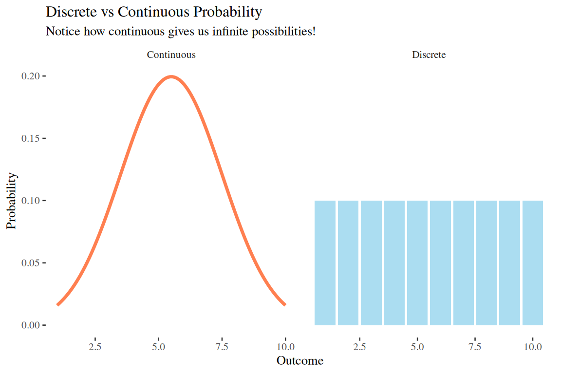
Think about it: Your height isn’t exactly 68 inches, it’s 68.2, 67.8, or 68.0000001 inches! The world around us is beautifully continuous, and we need powerful tools to understand it.
The Magic of Continuity:
Continuous random variables are the backbone of modeling real-world phenomena where outcomes can take any value within a range. Unlike discrete variables, which deal with countable outcomes, continuous variables are described by smooth curves called Probability Density Functions (PDFs).
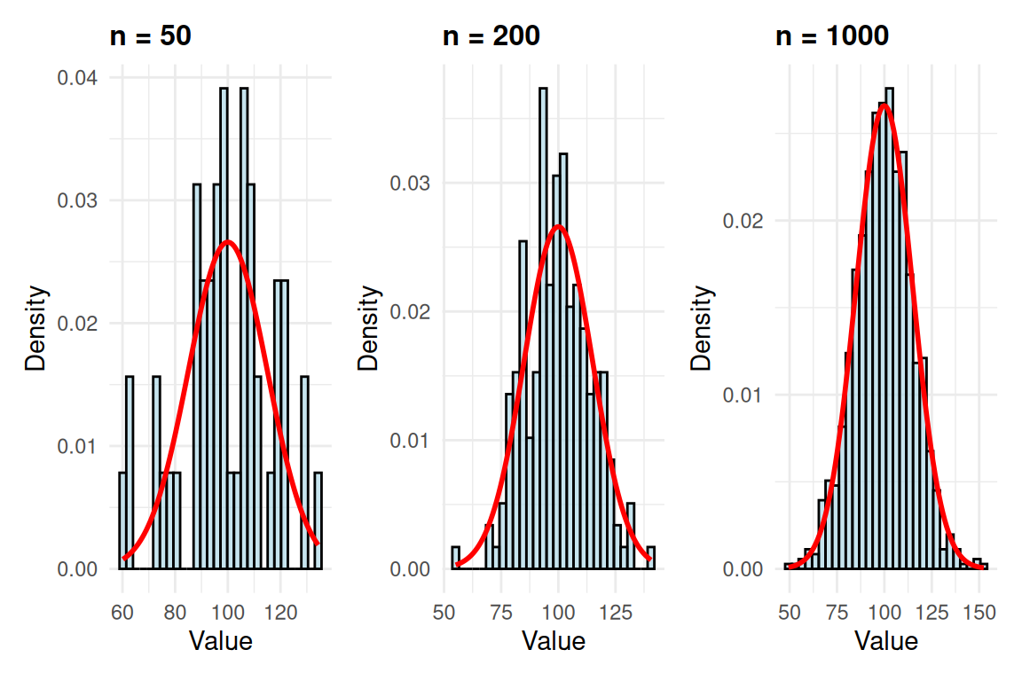
Empirical Probability: As we collect more data, our histogram approaches the true probability density function!
The Magic of Large Samples: Notice how n=1000 gives us a nearly perfect match to our theoretical curve.
Your Observation: What do you notice about the relationship between sample size and curve smoothness?
The Beautiful Connection: In continuous probability, we use calculus to find probabilities!
\[P(a \leq X \leq b) = \int_a^b f(x)\,dx\]
What this means: The probability equals the area under the curve between points a and b!
Definition
The uniform distribution models scenarios where every outcome in a range is equally likely. It’s the simplest continuous distribution, yet it’s incredibly useful in practice.
Why Use the Uniform Distribution?
Equal Likelihood:
It’s ideal for modeling fair processes.
Easy Calculations:
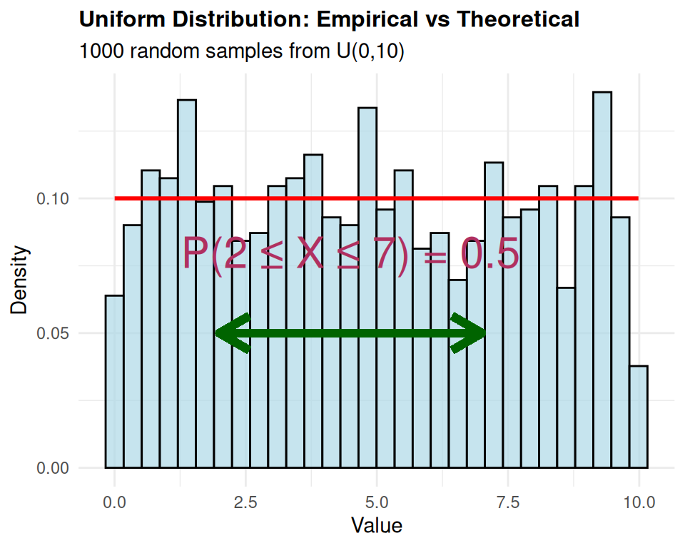
Probabilities are straightforward to compute. For example, \(P(a \leq X \leq b) = (b-a) \times \frac{1}{d-c}\).
Empirical Evidence:
Notice how our histogram matches the theoretical flat line
Mean and Median: Both are located at the center of the interval: \(\mu = \frac{a+b}{2}\).
Variance: The spread of the distribution is \(\sigma^2 = \frac{(b-a)^2}{12}\). A wider range leads to greater variability.
Empirical Verification: Try calculating these from our sample data above - do they match the theoretical values?