Day 15

Math 216: Statistical Thinking

Bastola

The Exponential Distribution: When Time Matters

Think about it: You’re waiting for the bus, your phone battery is dying, and you need to know - how long until the next one arrives? The exponential distribution is your crystal ball for waiting times!

Real-World Detective Work:

• Urban Planning: When will the next bus arrive?
• Tech Support: How long until your laptop crashes again?
• Emergency Services: When will the next 911 call come in?
• Quality Control: How long until this machine breaks down?

From Normal to Exponential: A New Type of Randomness

The Big Idea: Models waiting times between completely random events

Properties:

• Memoryless: Past waiting doesn’t affect future waiting
• Single Parameter: θ controls everything (mean = std dev!)
• Scale Matters: Larger θ = longer average waits

Detective’s Secret: If events happen randomly over time, waiting times follow exponential!

The Exponential Formula

Definition

The exponential distribution describes the time between events in a Poisson process, where events occur continuously and independently at a constant average rate.

Probability Density Function (PDF): \[f(x)=\frac{1}{\theta} \exp \left(-\frac{x}{\theta}\right), \quad x>0\]

• \(\theta\): Scale parameter (mean waiting time)
• \(x\): Waiting time between events
• Key Insight: The probability decays exponentially with time!

Statistical Measures

Key Parameters:

• Mean: \(\mu=\theta\) (Average waiting time)
• Rate: \(\lambda=\frac{1}{\theta}\) (Events per unit time)
• Standard Deviation: \(\sigma=\theta\) (Spread equals mean!)
• Variance: \(\sigma^2=\theta^2\)

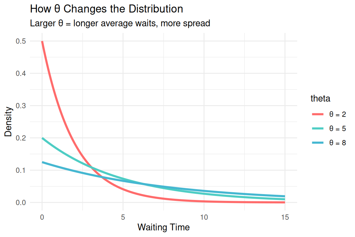
Real-World Interpretation:

• θ = 2 minutes: Buses arrive every 2 minutes on average
• θ = 5 hours: Equipment fails every 5 hours on average
• θ = 30 days: Customer complaints every 30 days on average

Calculating Probabilities

Probability Work:

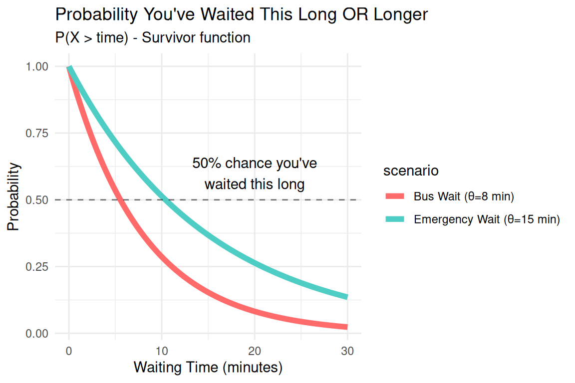
The Golden Formula: \(P(X \text{ > } a) = \exp\left(-\frac{a}{\theta}\right)\)

Bus Example (θ = 8 min):

• P(X > 5 min) = exp(-5/8) = 53.5%
• P(X > 15 min) = exp(-15/8) = 15.3%
• P(X > 30 min) = exp(-30/8) = 2.4%

Emergency Room (θ = 15 min):

• P(X > 10 min) = exp(-10/15) = 51.3%
• P(X > 30 min) = exp(-30/15) = 13.5%

Insight: Long waits become exponentially unlikely!

Calculating Probabilities and Quantiles in R

pexp: Calculates the cumulative probability for a given value.

• Syntax: pexp(q, rate = 1, lower.tail = TRUE)
• Computes \(P(X \leq x)\) or \(P(X > x)\) for an exponential distribution.
• Examples:
  • pexp(5, rate = 1/2) calculates \(P(X \leq 5)\) for \(\theta = 2\).
  • pexp(5, rate = 1/2, lower.tail = FALSE) for \(P(X > 5)\).

Calculating Probabilities and Quantiles in R

qexp: Computes the quantile for a specified probability.

• Syntax: qexp(p, rate = 1, lower.tail = TRUE)
• Finds the smallest \(x\) such that \(P(X \leq x) \geq p\).
• Examples:
  • qexp(0.7, rate = 1/2) finds the time by which 70% of events are expected to occur for \(\theta = 2\).

Geometric vs Exponential: The Connection

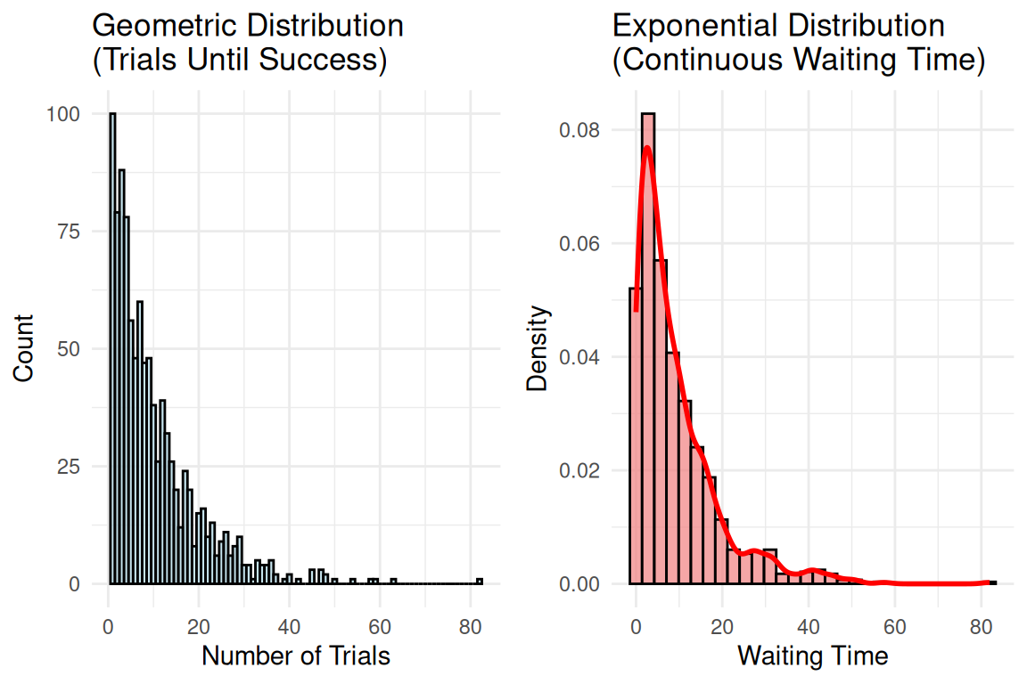
• Geometric: “How many resumes until I get a job offer?”
• Exponential: “How long until I get my next job offer?”

Geometric Distribution (Discrete Cousin)

• Counts: Number of trials until first success
• Examples: Coin flips, dice rolls, survey responses
• Memoryless: Past failures don’t affect future success

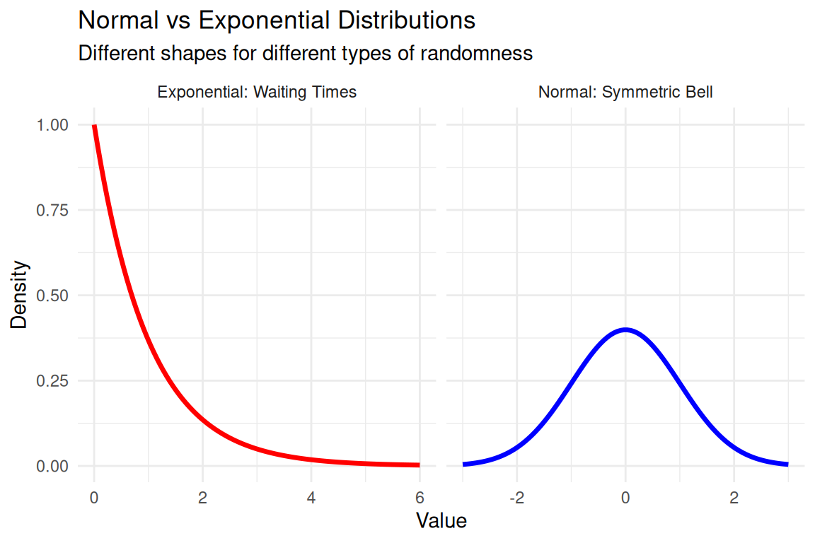
Exponential Distribution (Continuous Sibling)

• Measures: Continuous waiting time between events
• Examples: Time, distance, continuous measurements
• Memoryless: Past waiting doesn’t affect future waiting

Case 1: Coffee Shop Rush Hour

The Scenario: Starbucks manager wants to know staffing needs during morning rush

Data: Average time between customer orders = 2.5 minutes (θ = 2.5)

Questions:

# Coffee shop analysis
theta_coffee <- 2.5

# Q1: What's the probability a customer arrives within 1 minute?
p_within_1min <- pexp(1, rate = 1/theta_coffee)
sprintf("P(wait ≤ 1 min) = %.1f%%", p_within_1min * 100)

[1] "P(wait ≤ 1 min) = 33.0%"

# Q2: How long until 80% of customers have arrived?
time_80_percent <- qexp(0.8, rate = 1/theta_coffee)
sprintf("80%% arrive within %.1f minutes", time_80_percent)

[1] "80% arrive within 4.0 minutes"

# Q3: Probability of waiting more than 5 minutes for next customer?
p_over_5min <- pexp(5, rate = 1/theta_coffee, lower.tail = FALSE)
sprintf("P(wait > 5 min) = %.1f%%", p_over_5min * 100)

[1] "P(wait > 5 min) = 13.5%"

Manager’s Insight: Most customers arrive quickly, but occasional long gaps allow barista breaks!

Case 2: Tech Support Response Times

The Scenario: IT helpdesk promises 90% of tickets resolved within target time

Data: Historical average resolution time = 4.2 hours (θ = 4.2)

Investigation:

# Tech support analysis
theta_tech <- 4.2

# Q1: What time should we promise for 90% resolution?
promise_time <- qexp(0.9, rate = 1/theta_tech)
sprintf("Promise resolution within %.1f hours for 90%% success", promise_time)

[1] "Promise resolution within 9.7 hours for 90% success"

# Q2: What's the probability a ticket takes over 8 hours?
p_over_8hr <- pexp(8, rate = 1/theta_tech, lower.tail = FALSE)
sprintf("P(resolution > 8 hr) = %.1f%%", p_over_8hr * 100)

[1] "P(resolution > 8 hr) = 14.9%"

# Q3: Median resolution time?
median_time <- qexp(0.5, rate = 1/theta_tech)
sprintf("50%% of tickets resolved within %.1f hours", median_time)

[1] "50% of tickets resolved within 2.9 hours"

Service Level: Promise 9.7 hours for 90% success rate, but most tickets (50%) solved in 2.9 hours!

Case 3: Quality Control Testing

The Scenario: Manufacturing plant tests equipment reliability

Data: Average time between failures = 45 days (θ = 45)

Reliability Analysis:

# Quality control analysis
theta_equipment <- 45

# Q1: Probability equipment runs 30 days without failure?
p_30_days <- pexp(30, rate = 1/theta_equipment, lower.tail = FALSE)
sprintf("P(no failure for 30 days) = %.1f%%", p_30_days * 100)

[1] "P(no failure for 30 days) = 51.3%"

# Q2: Warranty period for 95% reliability?
warranty_95 <- qexp(0.95, rate = 1/theta_equipment)
sprintf("95%% reliable for %.1f days", warranty_95)

[1] "95% reliable for 134.8 days"

# Q3: Probability of failure in first week?
p_first_week <- pexp(7, rate = 1/theta_equipment)
sprintf("P(failure in first week) = %.1f%%", p_first_week * 100)

[1] "P(failure in first week) = 14.4%"

Quality Promise: Equipment is 95% reliable for 135 days - perfect for 4-month warranties!

R Functions: Your Statistical Calculator

pexp: “What’s the probability?”

• Syntax: pexp(q, rate = 1/θ, lower.tail = TRUE)
• Bus Example: pexp(5, rate = 1/8) = P(wait ≤ 5 minutes) = 46.5%
• Emergency: pexp(10, rate = 1/15) = P(wait ≤ 10 minutes) = 48.7%

qexp: “How long for this probability?”

• Syntax: qexp(p, rate = 1/θ, lower.tail = TRUE)
• Bus Example: qexp(0.9, rate = 1/8) = 90% of people wait ≤ 18.4 minutes
• Emergency: qexp(0.5, rate = 1/15) = 50% of patients wait ≤ 10.4 minutes

Shortcut: Use rate = 1/θ to convert from your average wait time!