Day 16
Math 216: Statistical Thinking
Bastola
The Sampling Distribution
Key Question: How can we estimate population characteristics from samples? Sampling distributions provide the theoretical foundation for statistical inference!
Real-World Applications:
- Political Polls: Predict elections from ~1,000 voters
- Medical Research: Test drug effectiveness on small patient cohorts
- Quality Control: Monitor product reliability without testing every item
- Market Research: Understand customer preferences from representative samples
Sampling Distribution
Key Insight: Population parameters are unknown - we can only observe samples!
Statistical Framework:
- 🔍 Sample Statistics: Estimates calculated from data
- 📊 Sampling Distributions: Patterns showing how estimates vary across samples
- 🎯 Parameter Estimation: Making inferences about population parameters
- ⚖️ Confidence Intervals: Quantifying uncertainty in our estimates
Fundamental Principle: Sample statistics follow predictable patterns - this enables population inference!
Sampling Distribution
The Concept of a Sampling Distribution
Definition
Sampling Distribution: The probability distribution of a statistic obtained from a large number of samples drawn from a specific population.
Key Components:
- Population Parameter: Fixed, unknown characteristic of the entire population (μ, σ)
- Sample Statistic: Estimate calculated from sample data (x̄, s)
- Sampling Distribution: Pattern showing how sample statistics vary across different samples
Key Insight: Even though each sample gives a different answer, they follow a predictable pattern!
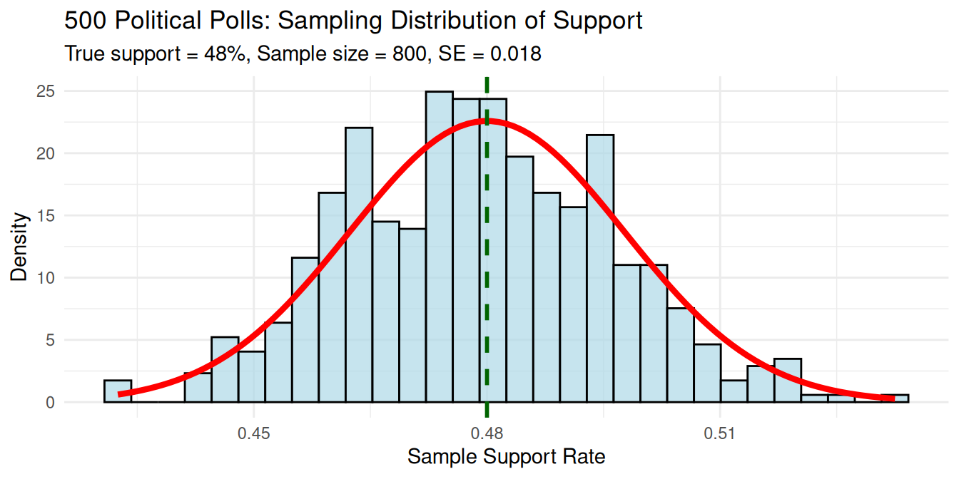
Case 1: Political Poll Analysis
Context: Predicting election results. True support = 48%, sample size = 800 voters.
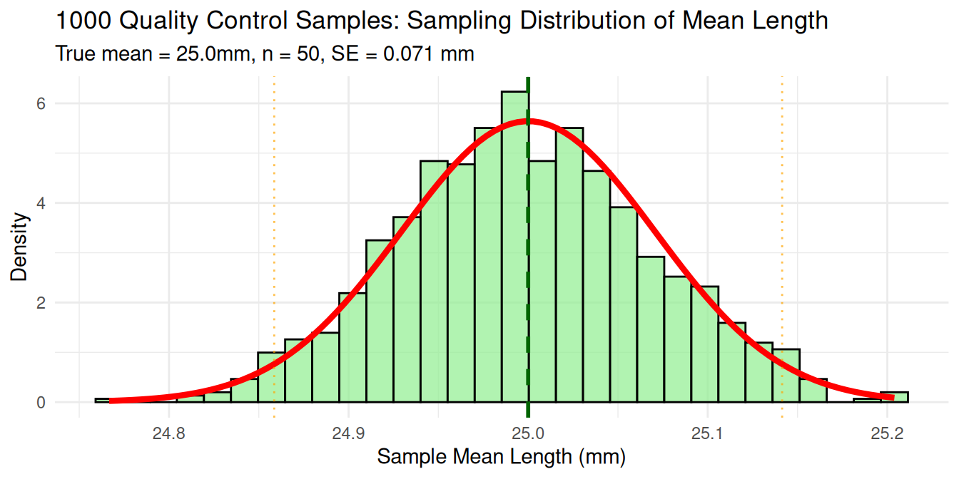
Case 2: Quality Control Analysis
Context: Factory produces bolts with true average length = 25.0mm. Quality control samples 50 bolts daily.
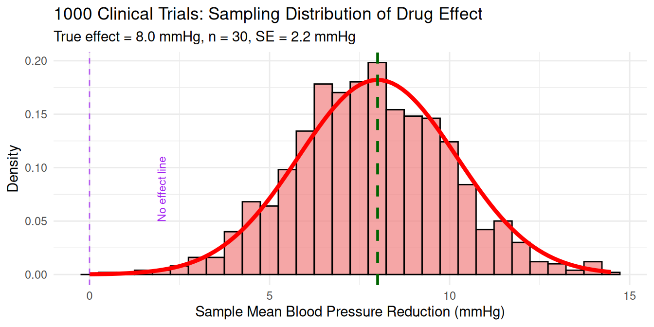
Case 3: Medical Research Analysis
Context: New drug lowers blood pressure by average of 8 mmHg. Clinical trial tests 30 patients.
Calculating Sample Statistics
Point Estimators:
- Sample Mean (\(\bar{x}\)): \(\bar{x}=\frac{\sum x_i}{n}\)
- Interpretation: Average of sample data
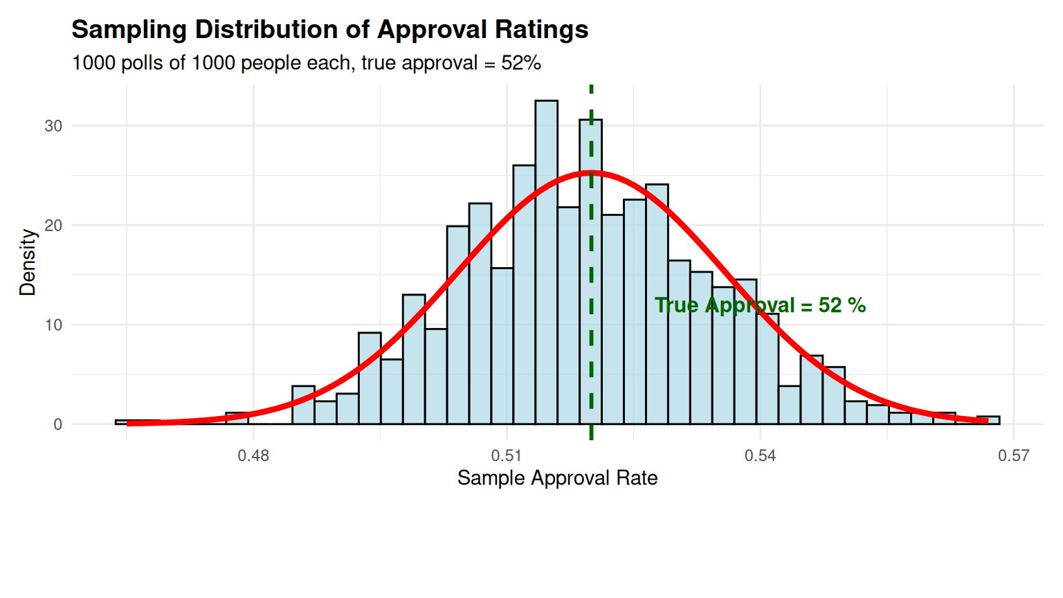
- Example: Average approval from 1000 poll respondents
- Sample Variance (\(s^2\)): \(s^2=\frac{\sum(x_i-\bar{x})^2}{n-1}\)
- Interpretation: Measure of data variability
- Example: Variability in drug response across 30 patients
Purpose: These estimators approximate unknown population parameters.
Key Insight: The sampling distribution shows the reliability of these estimates.
Unbiasedness and Minimum Variance
Unbiased Estimators:
- Definition: An estimator that consistently represents the population parameter across different samples
- Key Property: Expected value equals the population parameter
- Example: Sample mean (x̄) is unbiased for population mean (μ)
Minimum Variance
- Definition: Among unbiased estimators, prefer those with smaller variances
- Rationale: More precise estimates
- Example: Sample mean has smaller variance than sample median for normal data
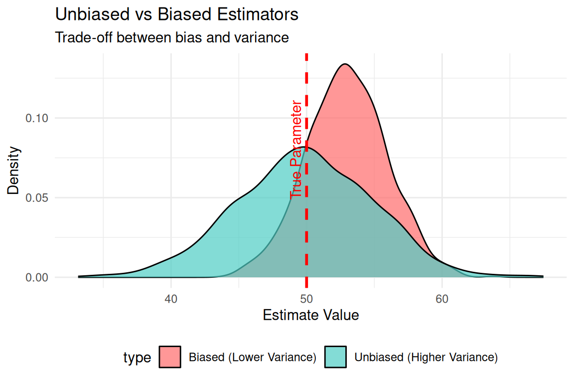
The Trade-off:
- Unbiased + High Variance: Sometimes far from truth, but correct on average
- Biased + Low Variance: Consistently wrong by same amount
- Ideal: Unbiased + Minimum Variance!
Statistical Principle: Prefer unbiased estimators with minimum variance.
Standard Error
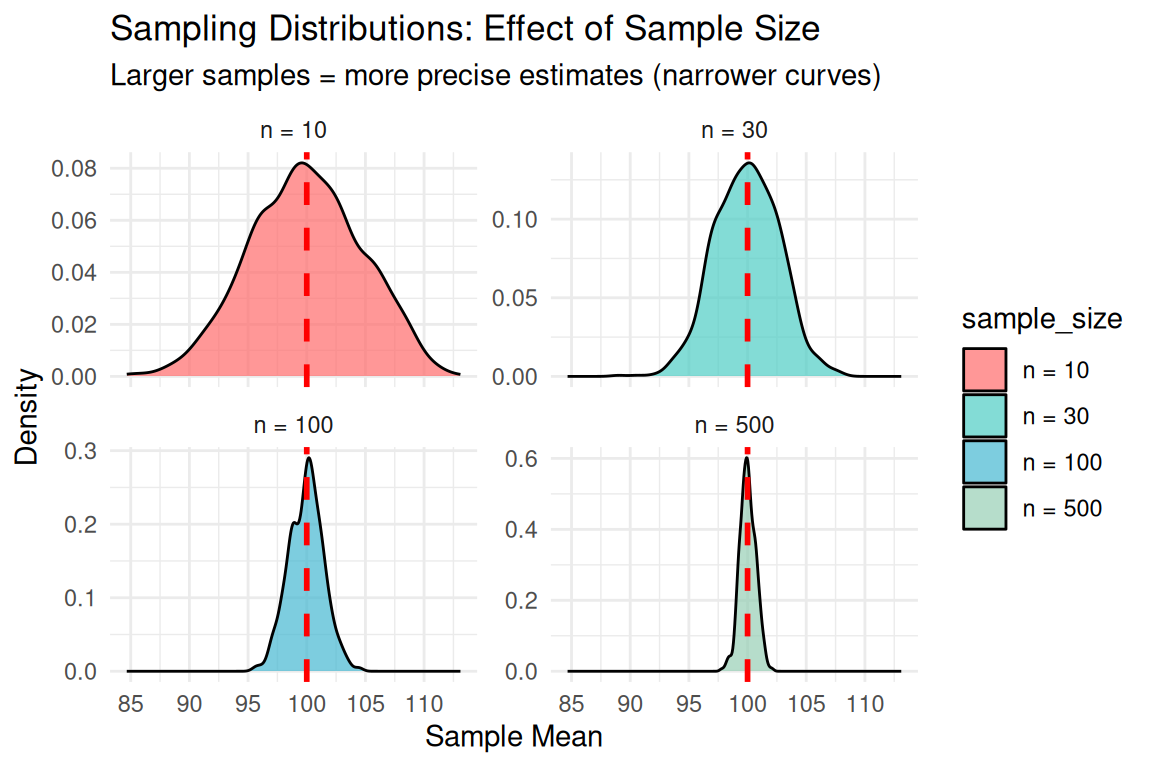
Standard Error
Standard Error Formula: \(SE = \frac{\sigma}{\sqrt{n}}\)
Interpretation by Sample Size:
- n = 10: High uncertainty, wide spread
- n = 30: Moderate uncertainty
- n = 100: Good precision
- n = 500: High precision, narrow spread
Key Principle: Larger samples = more precise estimates!
Mathematical Insight: Standard error decreases with √n, so quadrupling sample size halves the uncertainty!
Estimation Error: Confidence Level
Standard Error: How much sample statistics typically vary
- Example: Polls vary by ±3% from true approval rating
- Interpretation: Typical distance between sample and population
Estimation Error: How far off a single estimate probably is
- Example: Your poll shows 45%, but true support is probably 42-48%
- Interpretation: Uncertainty range around the estimate
The Relationship:
Estimation Error ≈ Standard Error × Critical Value (usually 1.96 for 95% confidence)
Interpretation: Quantifies confidence in estimates
Statistical Principle: Larger samples → smaller standard errors → more precise estimates!
Bias-Variance Tradeoff: Comparative Analysis
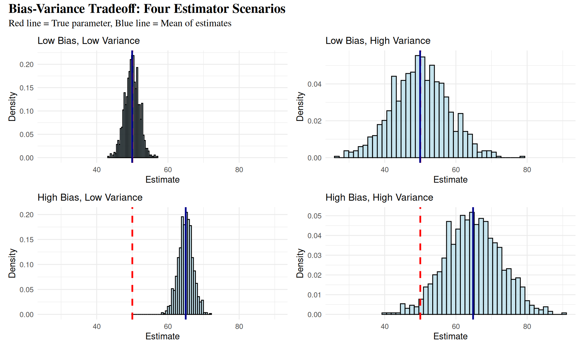
Key Insights from Bias-Variance Tradeoff
Top Row - Low Bias Estimators:
- Left: Ideal case - accurate and precise
- Right: Unbiased but imprecise - estimates vary widely
Bottom Row - High Bias Estimators:
- Left: Consistently wrong but precise
- Right: Worst case - inaccurate and imprecise
Statistical Principle: Seek estimators that balance bias and variance for optimal performance.