Day 17
Math 216: Statistical Thinking
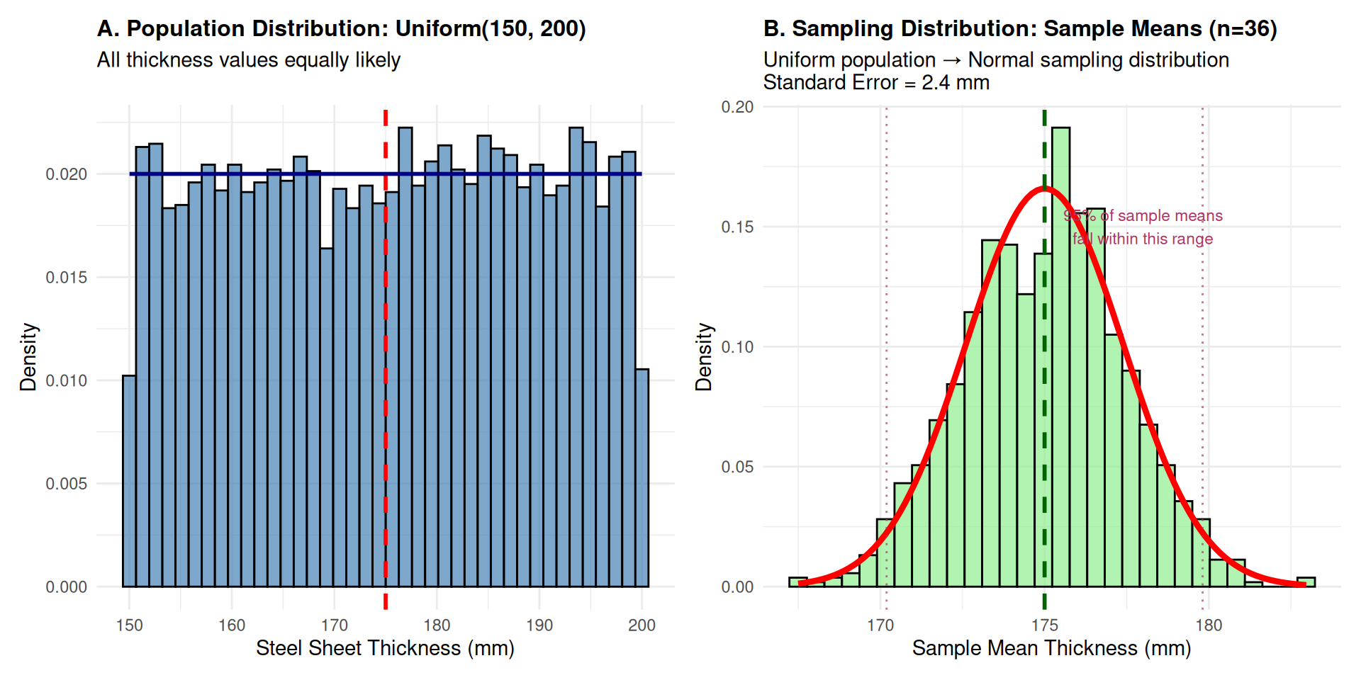
Case Study 1: Steel Manufacturing
Industrial Context: Steel sheets produced with uniform thickness distribution (150-200 mm). Quality assurance requires monitoring average thickness from small samples.
Case Study 2: Exponential Distribution Analysis
Context: Customer service call durations follow exponential distribution with mean = 5 minutes.
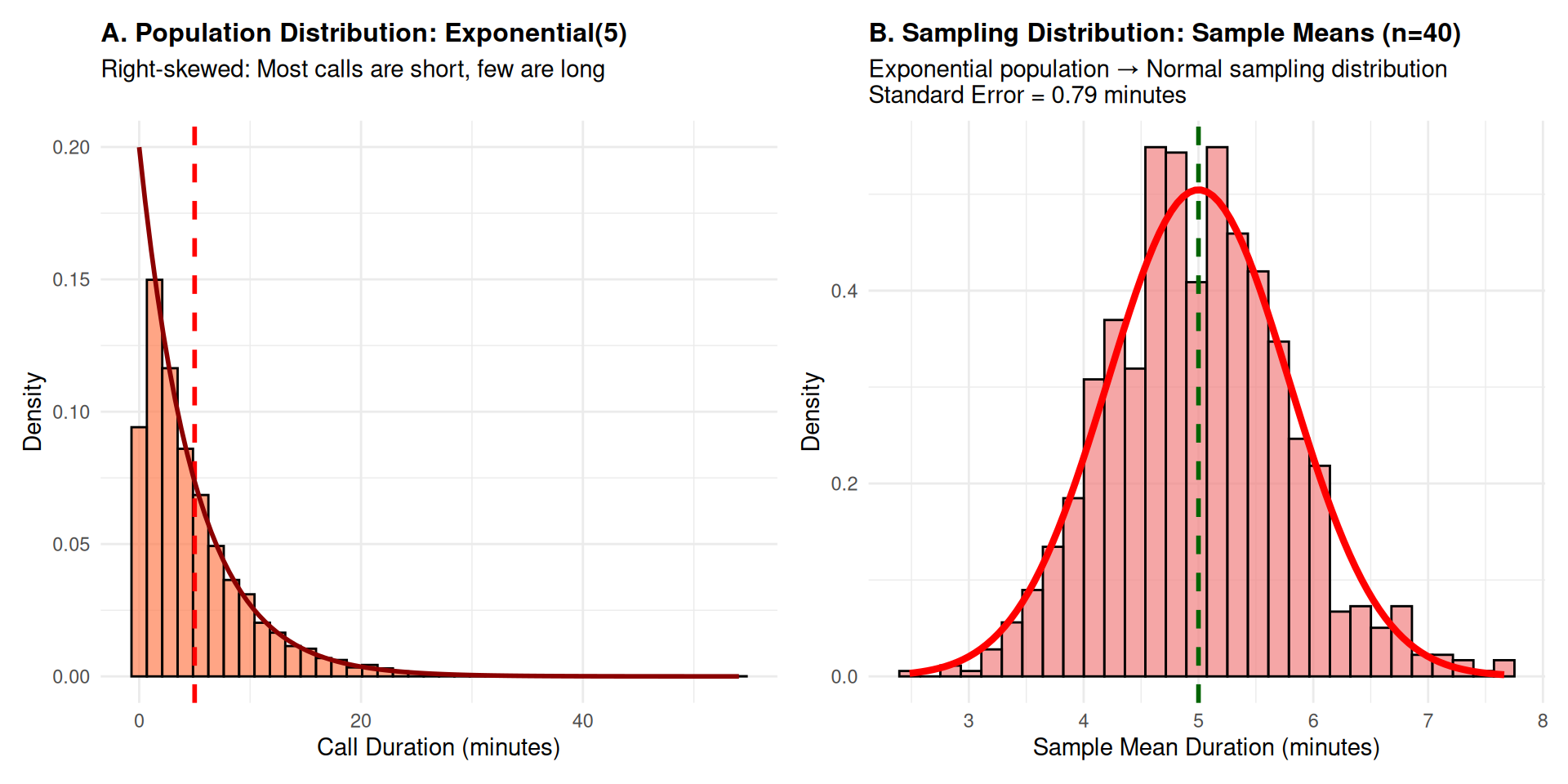
Statistical Insight: Even with highly skewed exponential population, sample means become normally distributed with n=40!
Case Study 3: Bimodal Distribution Analysis
Context: Product weights from two different production lines create bimodal distribution.
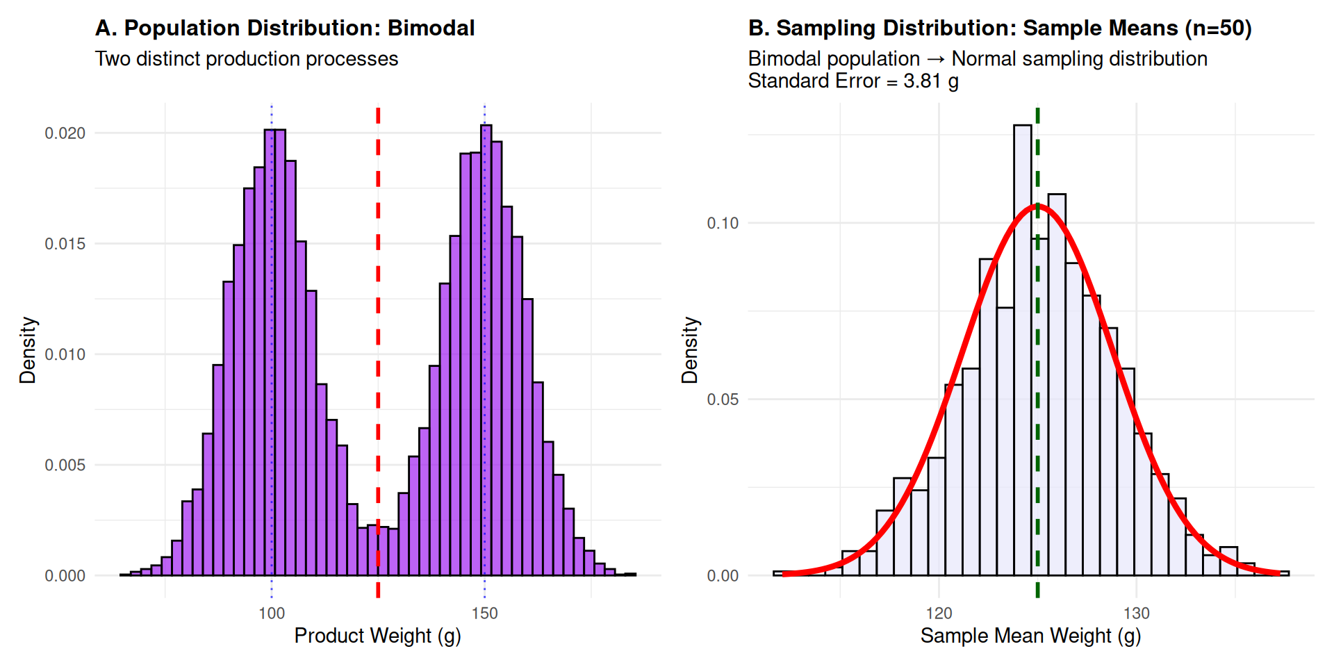
Statistical Insight: Complex bimodal populations still yield normally distributed sample means with adequate sample size!
Case Study 4: Left-Skewed Distribution Analysis
Context: Employee performance ratings with left-skewed distribution (most employees rated highly).
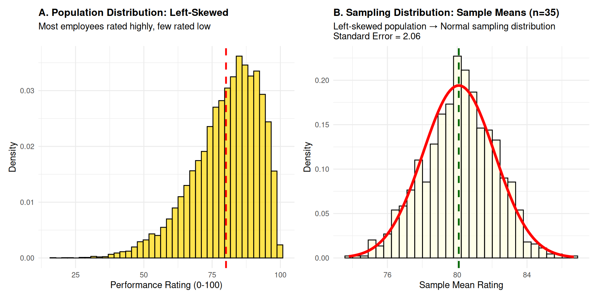
Statistical Insight: Left-skewed populations also produce normally distributed sample means with sufficient sample size!
Standard Error: Quantifying Estimation Precision
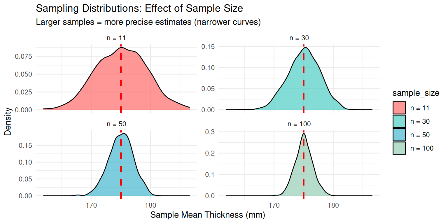
Standard Error Formula: \(SE = \frac{\sigma}{\sqrt{n}}\)
Applications of Central Limit Theorem: Political Polling
Context: Predicting election outcomes from voter samples
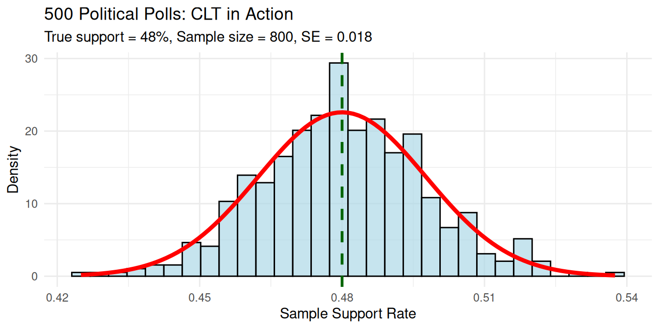
Statistical Findings:
- Poll results follow normal distribution despite binary data
- 95% of polls fall between 44.5% and 51.5%
- CLT enables accurate predictions from small samples
Applications of Central Limit Theorem: Quality Control
Context: Monitoring production quality from small samples
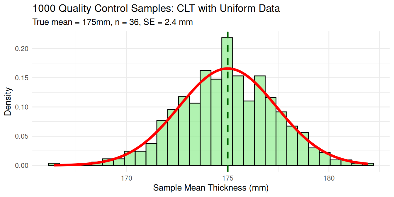
Quality Control Analysis:
- Uniform population → Normal sampling distribution
- 95% of samples fall within 174.3-175.7mm
- CLT works effectively with non-normal populations
Applications of Central Limit Theorem: Medical Research
Context: Testing drug effectiveness from clinical trials
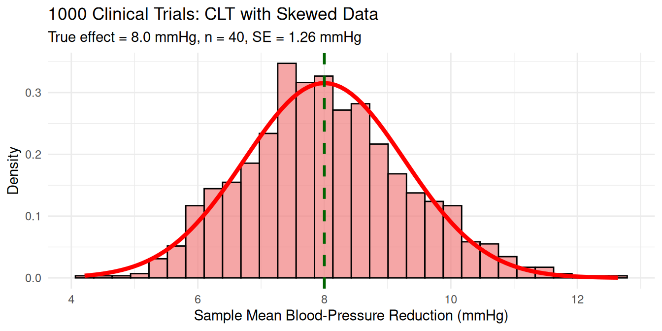
Medical Research Analysis:
- Skewed population → Normal sampling distribution
- CLT functions with any population shape
- Sample size is more critical than population distribution