Day 18
Math 216: Statistical Thinking
Sampling Distributions for Proportions: Statistical Inference Foundation
Key Question: How can we accurately estimate population proportions from sample data? Sampling distributions provide the theoretical framework for statistical inference with categorical data!
Real-World Applications:
- Political Polling: Estimate voter support from representative samples
- Market Research: Understand customer preferences and behaviors
- Quality Control: Monitor defect rates in manufacturing processes
- Medical Research: Track treatment success rates in clinical trials
Statistical Framework: From Population to Sample
Statistical Framework:
- 🎯 Population Proportion (p): True but unknown characteristic of entire population
- 🔍 Sample Proportion (\(\hat{p}\)): Estimate calculated from sample data
- 📊 Sampling Distribution: Pattern showing how \(\hat{p}\) varies across different samples
- ⚖️ Standard Error: Quantifies precision of our estimate
Key Insight: Even though each sample gives a different answer, they follow a predictable normal pattern!
Visualizing Sampling Distributions
Properties of Sampling Distribution
Core Statistical Properties
Mean of \(\hat{p}\):
- Unbiased Estimator: The expected value equals the population proportion
- Mathematical Form: \(E(\hat{p}) = \mu_{\hat{p}} = p\)
- Interpretation: On average, sample proportions equal the true population proportion
Standard Error of \(\hat{p}\):
- Precision Measure: Quantifies variability across different samples
- Mathematical Form: \(\sigma_{\hat{p}} = \sqrt{\frac{p(1-p)}{n}}\)
- Interpretation: Larger samples → smaller standard error → more precise estimates
Key Insight: These properties enable statistical inference from samples to populations!
Central Limit Theorem for Proportions
Core Statistical Principle
Central Limit Theorem for Proportions: For sufficiently large samples, the sampling distribution of \(\hat{p}\) is approximately normal, regardless of the population distribution shape.
Mathematical Formulation: \[\hat{p} \sim N\left(p, \sqrt{\frac{p(1-p)}{n}}\right)\]
Sample Size Requirements:
- Success-Failure Condition: \(np \geq 15\) and \(n(1-p) \geq 15\)
- Practical Interpretation: Ensure enough successes and failures for normal approximation
Statistical Significance: This universal principle enables confidence intervals and hypothesis testing for proportions!
CLT Condition Verification
Central Limit Theorem Conditions
Success-Failure Condition: For normal approximation to be valid, we need: \[np \geq 15 \quad \text{and} \quad n(1-p) \geq 15\]
Verification Examples:
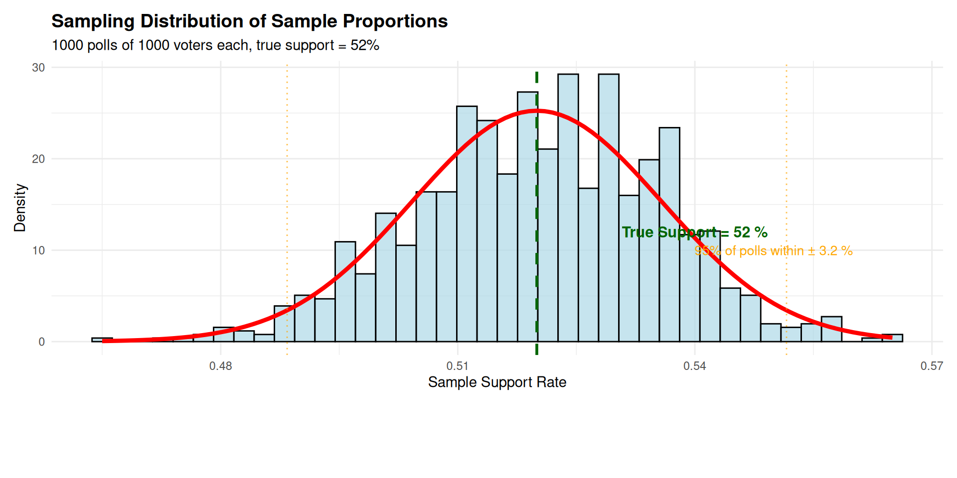
Example 1: Political Polling
- Population proportion: \(p = 0.52\) (52% support)
- Sample size: \(n = 1000\)
- \(np = 1000 \times 0.52 = 520 \geq 15\) ✅
- \(n(1-p) = 1000 \times 0.48 = 480 \geq 15\) ✅
- Conclusion: CLT applies, normal approximation valid
Example 2: Market Research
- Population proportion: \(p = 0.30\) (30% preference)
- Sample size: \(n = 100\)
- \(np = 100 \times 0.30 = 30 \geq 15\) ✅
- \(n(1-p) = 100 \times 0.70 = 70 \geq 15\) ✅
- Conclusion: CLT applies, normal approximation valid
Z-Scores and Probability Calculations: Statistical Inference Tools
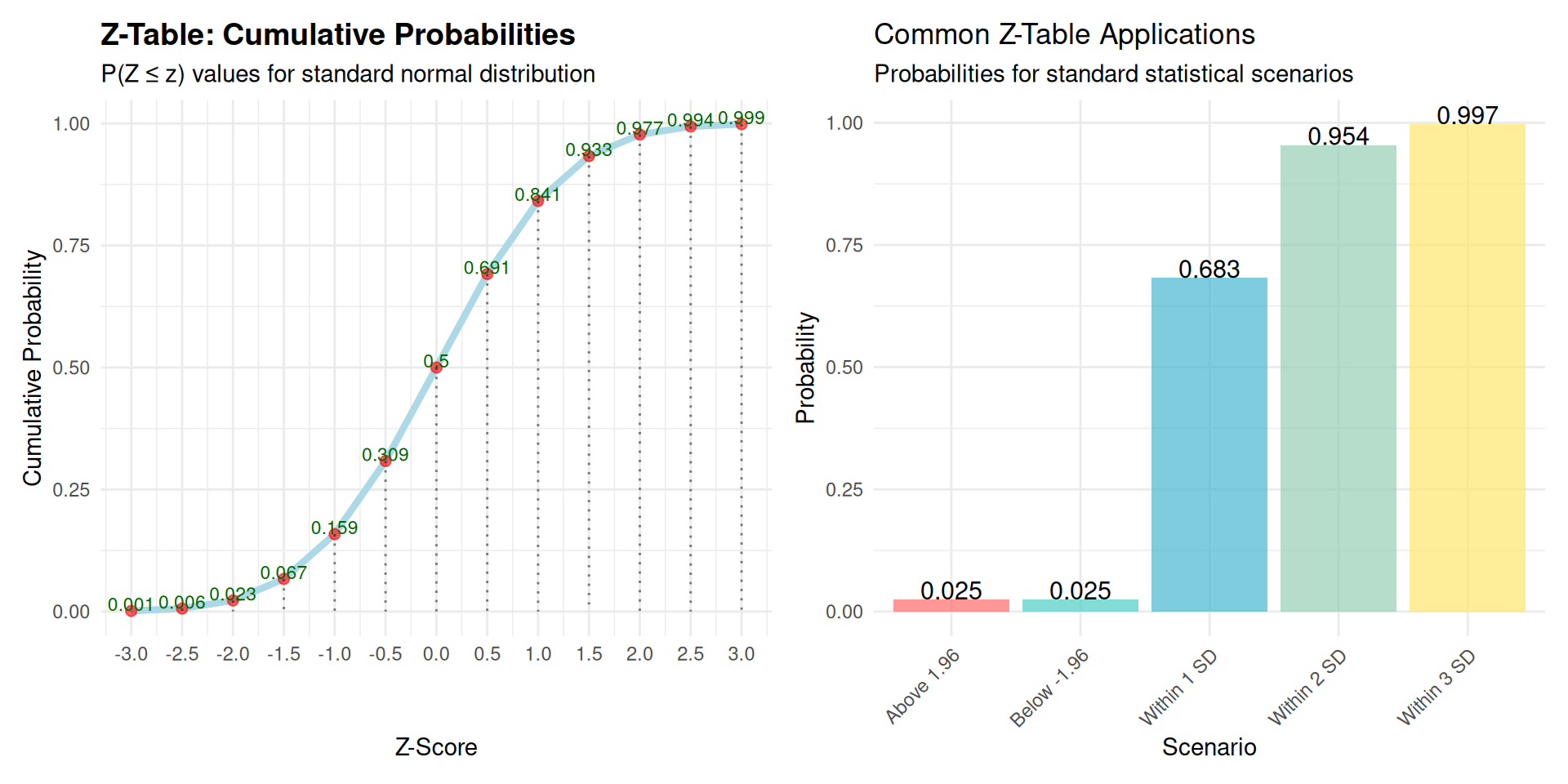
Z-Tables: Traditional Probability Calculation
Sampling Distribution Simulator
Probability Calculations
Probability Calculation Exercises
Real-World Application
Population proportion: \(p = 0.45\), sample size: \(n = 400\)
Standard error: \(SE = \sqrt{\frac{0.45 \times 0.55}{400}} = 0.0249\)
Find \(P(\hat{p} < 0.40)\):
pnorm((0.40-0.45)/0.0249) = 0.0222Find \(P(\hat{p} > 0.50)\):
1 - pnorm((0.50-0.45)/0.0249) = 0.0222Find \(P(0.42 < \hat{p} < 0.48)\):
pnorm((0.48-0.45)/0.0249) - pnorm((0.42-0.45)/0.0249) = 0.7699