| Parameter | Key Words or Phrases | Type of Data |
|---|---|---|
| \(\mu\) | Mean; average | Quantitative |
| \(p\) | Proportion; percentage; fraction; rate | Qualitative |
| \(\sigma^2\) (optional) | Variance; variability; spread | Quantitative |
Day 19
Math 216: Statistical Thinking
Bastola
Statistical Estimation: Bridging Samples and Populations
Key Question: How can we use sample data to make reliable inferences about unknown population parameters? Statistical estimation provides the mathematical framework for quantifying uncertainty in our conclusions!
Real-World Applications:
- Medical Research: Estimate treatment effects from clinical trial data
- Market Analysis: Determine consumer preferences from survey samples
- Quality Control: Monitor production processes using sample measurements
- Environmental Science: Assess pollution levels from limited monitoring stations
Target Parameters
Types of Statistical Estimators
Statistical Estimation Framework
Point Estimator: A single value that provides our best guess for the population parameter
- Example: \(\bar{x} = \frac{1}{n} \sum_{i=1}^n x_i\) estimates the population mean \(\mu\)
- Properties: Unbiased, consistent, efficient
Interval Estimator (Confidence Interval): A range of plausible values that likely contains the true parameter
- Mathematical Form: \(\text{Estimate} \pm \text{Margin of Error}\)
- Interpretation: Quantifies uncertainty in our estimation process
Key Insight: While point estimates give us a single “best guess,” confidence intervals provide the precision and reliability of that guess!
The Power of Confidence Intervals: Quantifying Uncertainty
Why Confidence Intervals Matter
Beyond Point Estimates: Confidence intervals provide more information than single values—they quantify the precision and reliability of our estimates!
Key Benefits:
- Uncertainty Quantification: Express the range of plausible values for the parameter
- Statistical Precision: Wider intervals indicate more uncertainty, narrower intervals indicate greater precision
- Decision Support: Help determine if effects are practically significant
- Method Reliability: The confidence level indicates how often the method produces intervals containing the true parameter
Statistical Significance: Confidence intervals are the foundation for hypothesis testing and statistical inference!
Calculating a Confidence Interval
- Scenario: Estimating average hospital stay length.
- Sample Data: Sample mean \(\bar{x}\) from 100 patient records.
- Central Limit Theorem: Assures that \(\bar{x}\) is approximately normally distributed for large samples.
Confidence Interval Formula
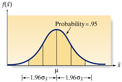
- 95% Confidence Interval for \(\mu\): \[ 95\% \text{ C.I.} = \left(\bar{x} - 1.96 \frac{\sigma}{\sqrt{n}}, \quad \bar{x} + 1.96 \frac{\sigma}{\sqrt{n}}\right) \]
- Note: \(\sigma\) is the standard deviation of the population, and \(n\) is the sample size.
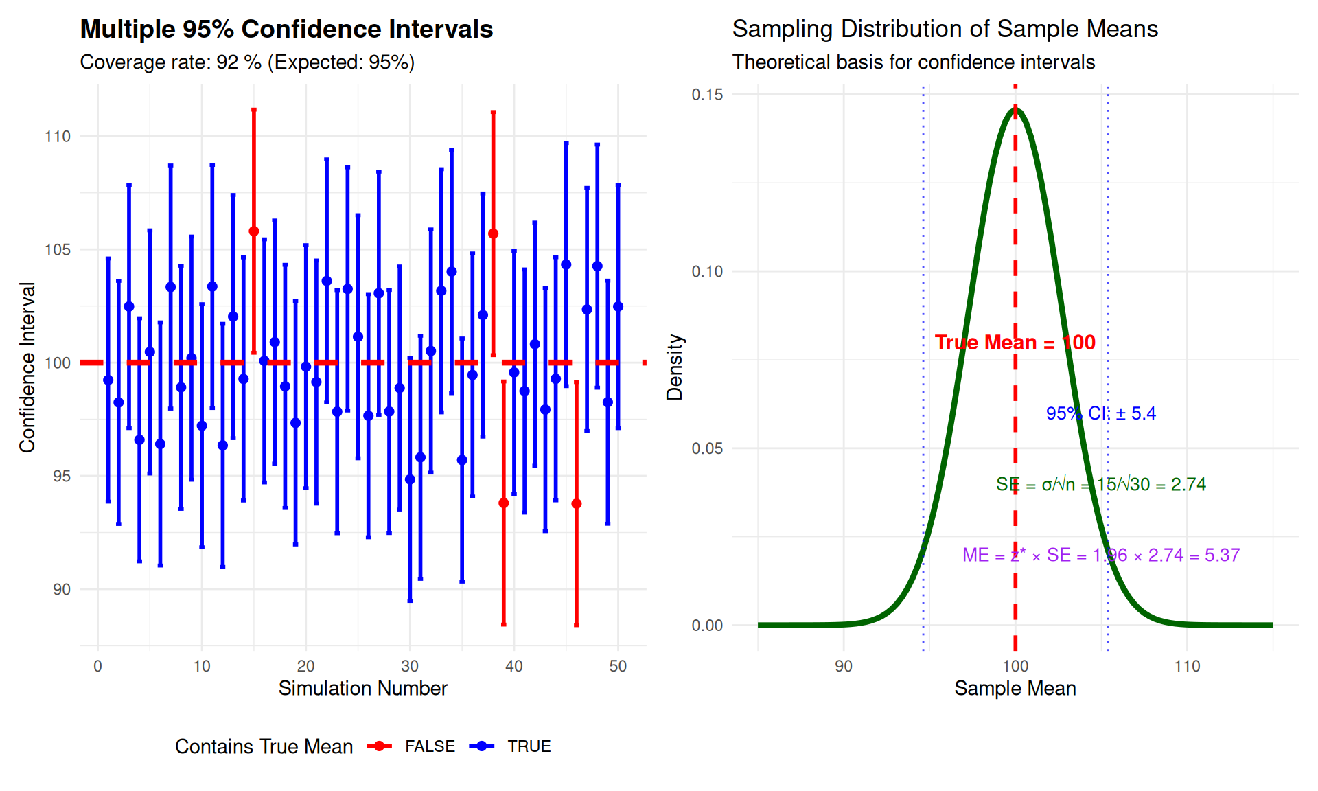
Understanding Confidence Intervals
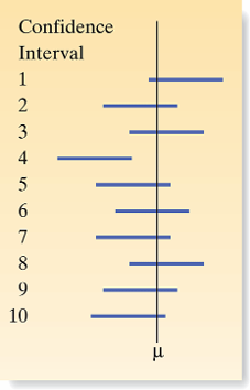
- Question: Is the true mean \(\mu\) between 3.81 and 5.25?
- Confidence Understanding:
- No certainty that \(\mu\) lies within this specific interval from a single sample.
- If repeated samples are taken, about 95% of such intervals would contain \(\mu\).
- Correct Interpretation:
- We don’t say \(\mu\) is definitely in this interval based on one sample; the 95% level reflects how often these intervals capture \(\mu\) across many samples.
- Terminology:
- Confidence Coefficient (.95): Proportion of intervals that will contain \(\mu\) over repeated sampling.
- Confidence Level (95%): Indicates method reliability over many trials.
Understanding CIs
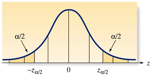
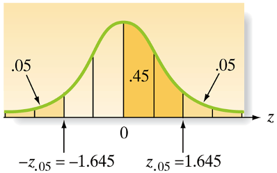
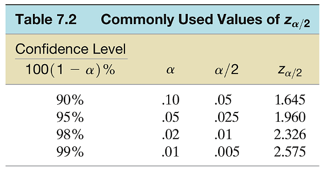
Commonly used values of \(z_{\alpha}\)
The value \(z_\alpha\) is defined as the value of the standard normal random variable \(z\) such that the area \(\alpha\) will lie to its right. In other words, \(P\left(z>z_\alpha\right)=\alpha\).
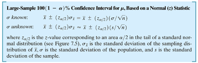
Large Sample Confidence Interval for \(\mu\)
Confidence Interval Visualization
Theoretical Calculations: pnorm and qnorm Applications
R Functions for Confidence Interval Calculations
Critical Value Calculations:
- 90% confidence:
qnorm(0.95) = 1.645 - 95% confidence:
qnorm(0.975) = 1.960 - 99% confidence:
qnorm(0.995) = 2.576
Probability Calculations:
- Probability within 1 SD:
pnorm(1) - pnorm(-1) = 0.6827 - Probability within 2 SD:
pnorm(2) - pnorm(-2) = 0.9545 - Probability within 3 SD:
pnorm(3) - pnorm(-3) = 0.9973
Confidence Interval Formula: \[\text{CI} = \bar{x} \pm z_{\alpha/2} \cdot \frac{\sigma}{\sqrt{n}}\]
Margin of Error: \[\text{ME} = z_{\alpha/2} \cdot \frac{\sigma}{\sqrt{n}}\]
Confidence Interval Exercises
Practical Exercises Using R
Exercise 1: Basic Confidence Interval Calculation
- Sample mean: 85, population SD: 12, sample size: 64
- Calculate 95% CI:
85 ± 1.96 * (12/sqrt(64)) = (82.06, 87.94) - R code:
85 + c(-1,1) * qnorm(0.975) * 12/sqrt(64)
Exercise 2: Sample Size Determination
- Desired margin of error: 2, population SD: 10, 95% confidence
- Required sample size:
n = (1.96 * 10 / 2)^2 = 96.04 → 97 - R code:
ceiling((qnorm(0.975) * 10 / 2)^2)
Confidence Interval Exercises
Practical Exercises Using R
Exercise 3: Confidence Level Impact
- Same data: mean=50, SD=8, n=36
- 90% CI:
50 ± 1.645*(8/6) = (47.81, 52.19) - 95% CI:
50 ± 1.96*(8/6) = (47.39, 52.61) - 99% CI:
50 ± 2.576*(8/6) = (46.57, 53.43)
Exercise 4: Real-World Interpretation
- Medical study: Treatment reduces blood pressure by 8 mmHg (95% CI: 5 to 11 mmHg)
- Interpretation: We’re 95% confident the true reduction is between 5 and 11 mmHg
- Statistical significance: Interval doesn’t include 0 → effect is statistically significant