Day 20
Math 216: Statistical Thinking
Challenges with Small Samples: Statistical Limitations
Small Sample Statistical Challenges
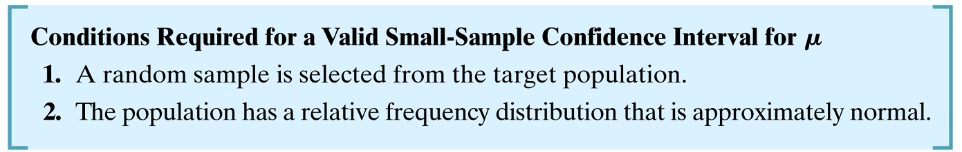
Normality Assumption: With samples smaller than 30, the Central Limit Theorem may not apply effectively, requiring the population distribution to be approximately normal for valid inference.
Standard Deviation Uncertainty: Using sample standard deviation \(s\) instead of population \(\sigma\) introduces additional variability that must be accounted for in our calculations.
Key Statistical Issues:
- Increased Variability: Small samples lead to greater uncertainty in parameter estimates
- Distribution Sensitivity: Results become more sensitive to the underlying population distribution
- Confidence Interval Width: Intervals become wider to account for increased uncertainty
Statistical Significance: These challenges necessitate specialized methods like the t-distribution for valid small-sample inference!
Small Sample Confidence Intervals
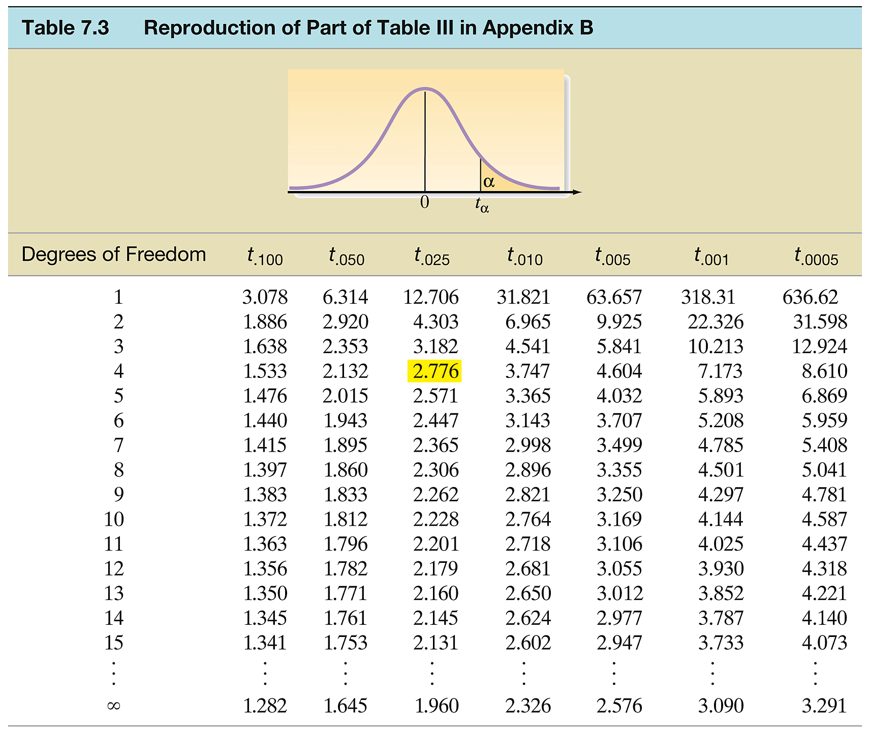
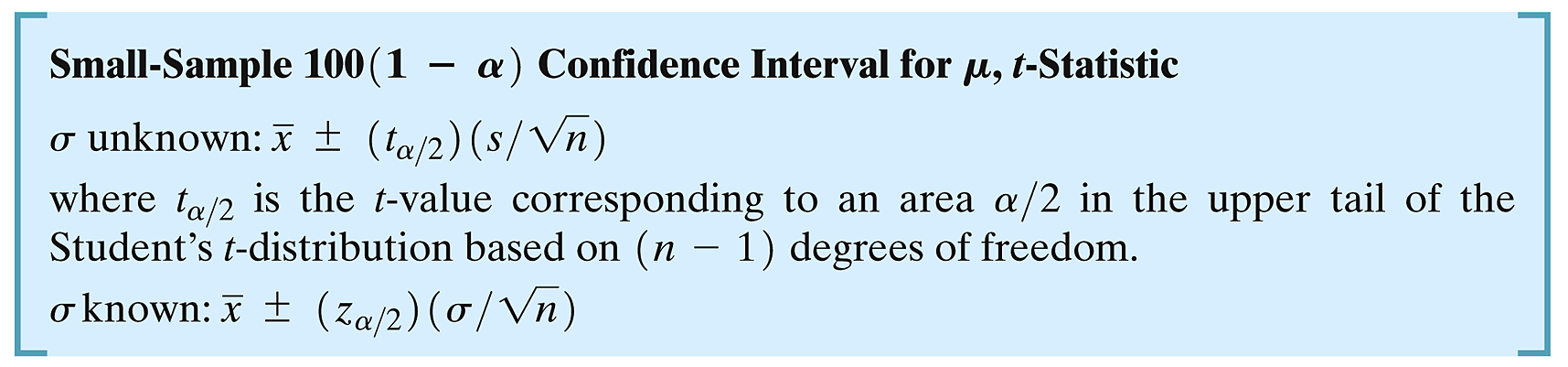
For small samples where the population standard deviation is unknown, we use the t-distribution to construct confidence intervals: \[ \bar{x} \pm t_{\alpha/2, df} \cdot \frac{s}{\sqrt{n}} \] This formula accounts for the additional uncertainty inherent in small samples.
Degrees of Freedom (df)
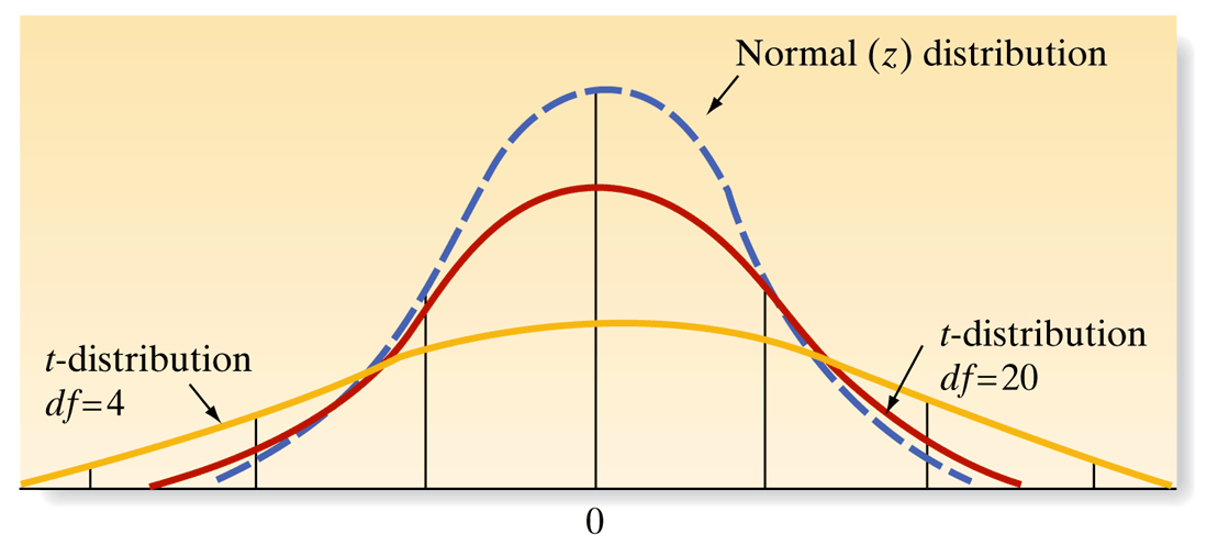
- Degrees of Freedom: The shape of the t-distribution and its variability depend on the degrees of freedom (df = \(n-1\)), which adjusts as the sample size changes. This flexibility makes it particularly useful for small sample sizes.
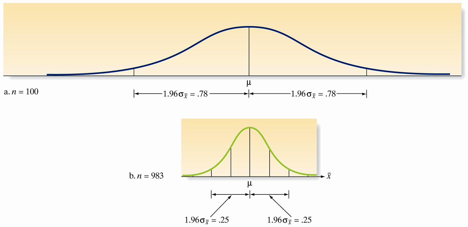
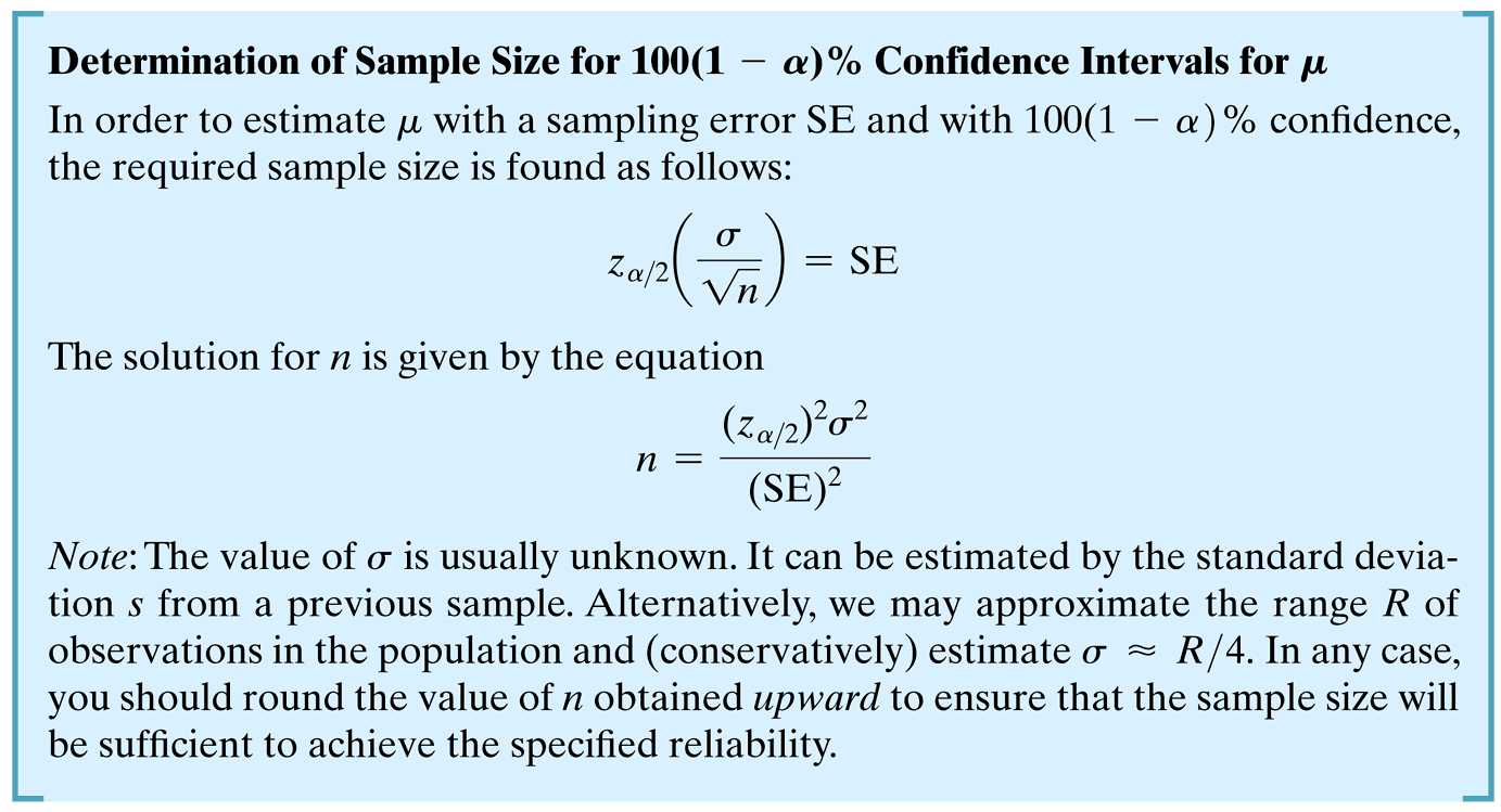
Overview of Determining Sample Size
- Importance of sample size in designing experiments.
- Impacts the reliability of inferences about a population mean.
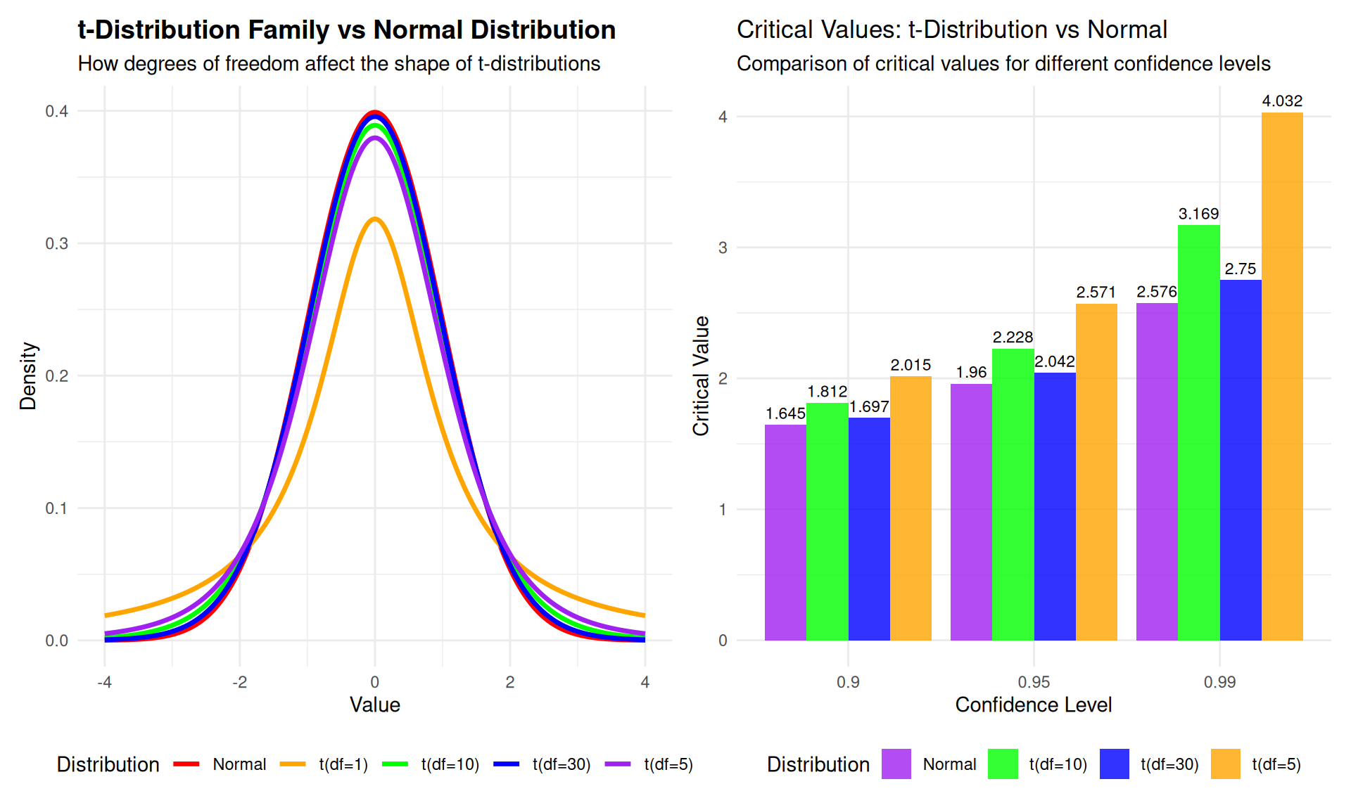
t-Distribution Visualization
Theoretical Calculations for Confidence Intervals
R Functions for Confidence Interval Calculations
Critical Value Calculations for 95% Confidence Intervals:
- Normal distribution (large samples):
qnorm(0.975) = 1.960 - t-distribution (df=10):
qt(0.975, df=10) = 2.228 - t-distribution (df=5):
qt(0.975, df=5) = 2.571 - t-distribution (df=2):
qt(0.975, df=2) = 4.303
Confidence Interval Formulas:
- Large sample: \(\bar{x} \pm z_{\alpha/2} \cdot \frac{s}{\sqrt{n}}\)
- Small sample: \(\bar{x} \pm t_{\alpha/2, df} \cdot \frac{s}{\sqrt{n}}\)
Key Insight: As degrees of freedom increase, t-distribution approaches normal distribution, and confidence intervals become narrower for the same confidence level!
Practical Interpretation:
- Higher critical values for small samples reflect greater uncertainty
- Wider intervals for small samples provide more conservative estimates
- The t-distribution automatically adjusts for sample size through degrees of freedom
t-Distribution Exercises and Applications
Practical Exercises Using R
Exercise 1: t-Distribution Critical Values for Confidence Intervals
- 95% CI, df=8:
qt(0.975, df=8) = 2.306 - 99% CI, df=15:
qt(0.995, df=15) = 2.947 - 90% CI, df=20:
qt(0.95, df=20) = 1.725
Exercise 2: Small Sample Confidence Interval Calculation
- Data: mean=50, SD=8, n=10
- 95% CI: \(50 \pm 2.262 \times (8/\sqrt{10}) = (44.28, 55.72)\)
- R code:
50 + c(-1,1) * qt(0.975, df=9) * 8/sqrt(10)
Exercise 3: Confidence Interval Width Comparison
- Compare 95% CI widths for different sample sizes using t-distribution
- n=5: width = \(2 \times 2.776 \times (8/\sqrt{5}) = 19.87\)
- n=10: width = \(2 \times 2.262 \times (8/\sqrt{10}) = 11.44\)
- n=20: width = \(2 \times 2.093 \times (8/\sqrt{20}) = 7.49\)
Real-World Confidence Interval Applications
Practical Applications Using t-Distribution
Application 1: Medical Research Interpretation
- Medical study: New drug reduces symptoms by 3.2 points (95% CI: 1.1 to 5.3, n=18)
- Interpretation: Using t-distribution (df=17), we’re 95% confident the true effect is between 1.1 and 5.3
- The interval provides a range of plausible values for the true treatment effect
Application 2: Environmental Monitoring
- Water quality study: Mean pollutant level = 12.5 ppm (95% CI: 8.2 to 16.8, n=8)
- Interpretation: We’re 95% confident the true mean pollutant level is between 8.2 and 16.8 ppm
- The wide interval reflects the uncertainty from small sample size
Application 3: Quality Control
- Manufacturing process: Mean dimension = 25.1 mm (95% CI: 24.8 to 25.4, n=6)
- Interpretation: We’re 95% confident the true mean dimension is between 24.8 and 25.4 mm
- The narrow interval suggests good process control despite small sample