Day 21
Math 216: Statistical Thinking
Confidence Intervals for Proportions: Statistical Inference Foundation
Key Question: How can we estimate population proportions with quantified uncertainty? Confidence intervals provide the mathematical framework for making reliable inferences about categorical data!
Real-World Applications:
- Political Polling: Estimate voter support with margin of error
- Market Research: Determine customer preference rates with confidence
- Quality Control: Monitor defect rates in manufacturing processes
- Medical Research: Track treatment success rates in clinical trials
- Public Health: Estimate disease prevalence from survey samples
Statistical Framework: From Sample to Population
Statistical Framework:
- 🎯 Population Proportion (p): True but unknown characteristic of entire population
- 🔍 Sample Proportion (\(\hat{p}\)): Estimate calculated from sample data
- 📊 Sampling Distribution: Pattern showing how \(\hat{p}\) varies across different samples
- ⚖️ Confidence Interval: Range of plausible values for the true population proportion
Key Insight: Confidence intervals quantify the precision of our estimates and provide a range of plausible values for the true population proportion!
Visualizing Sampling Distributions for Proportions
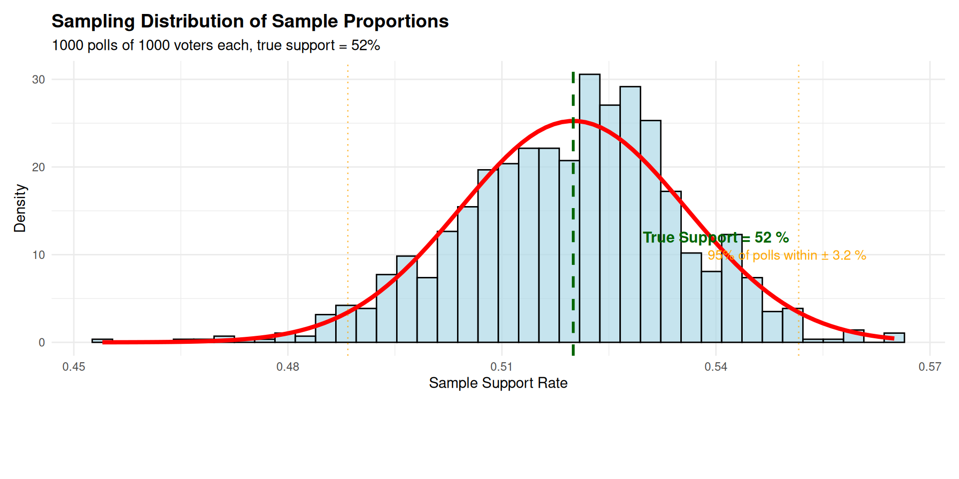
Properties of Sampling Distribution for Proportions
Core Statistical Properties
Mean of \(\hat{p}\):
- Unbiased Estimator: The expected value equals the population proportion
- Mathematical Form: \(E(\hat{p}) = \mu_{\hat{p}} = p\)
- Interpretation: On average, sample proportions equal the true population proportion
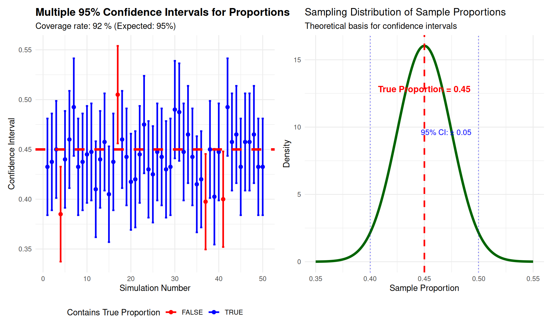
Standard Error of \(\hat{p}\):
- Precision Measure: Quantifies variability across different samples
- Mathematical Form: \(\sigma_{\hat{p}} = \sqrt{\frac{p(1-p)}{n}}\)
- Interpretation: Larger samples → smaller standard error → more precise estimates
Key Insight: These properties enable statistical inference from samples to populations!
Central Limit Theorem for Proportions
Core Statistical Principle
Central Limit Theorem for Proportions: For sufficiently large samples, the sampling distribution of \(\hat{p}\) is approximately normal, regardless of the population distribution shape.
Mathematical Formulation: \[\hat{p} \sim N\left(p, \sqrt{\frac{p(1-p)}{n}}\right)\]
Sample Size Requirements:
- Success-Failure Condition: \(np \geq 15\) and \(n(1-p) \geq 15\)
- Practical Interpretation: Ensure enough successes and failures for normal approximation
Statistical Significance: This universal principle enables confidence intervals and hypothesis testing for proportions!
Large-Sample Confidence Interval for \(p\)
Confidence Interval Formula
General Formula: \[\hat{p} \pm z_{\alpha/2} \sqrt{\frac{\hat{p}(1-\hat{p})}{n}}\]
Components:
- \(\hat{p} = \frac{x}{n}\): Sample proportion (successes/total)
- \(z_{\alpha/2}\): Critical value from standard normal distribution
- \(\sqrt{\frac{\hat{p}(1-\hat{p})}{n}}\): Standard error of \(\hat{p}\)
Common Confidence Levels:
- 90% confidence: \(z_{0.05} = 1.645\)
- 95% confidence: \(z_{0.025} = 1.960\)
- 99% confidence: \(z_{0.005} = 2.576\)
Key Insight: This formula provides a range of plausible values for the true population proportion!
Conditions for Valid Large-Sample C.I. for \(\boldsymbol{p}\)
Statistical Assumptions
Essential Conditions:
- Random Sample: Data collected through random sampling from target population
- Independence: Individual observations are independent of each other
- Success-Failure Condition: \(n\hat{p} \geq 15\) and \(n(1-\hat{p}) \geq 15\)
Verification Examples:
Example 1: Political Polling
- Sample size: \(n = 1000\), observed support: \(\hat{p} = 0.52\)
- \(n\hat{p} = 1000 \times 0.52 = 520 \geq 15\) ✅
- \(n(1-\hat{p}) = 1000 \times 0.48 = 480 \geq 15\) ✅
- Conclusion: Conditions satisfied, CI valid
Example 2: Market Research
- Sample size: \(n = 100\), preference rate: \(\hat{p} = 0.30\)
- \(n\hat{p} = 100 \times 0.30 = 30 \geq 15\) ✅
- \(n(1-\hat{p}) = 100 \times 0.70 = 70 \geq 15\) ✅
- Conclusion: Conditions satisfied, CI valid
Confidence Interval Visualization
Case Study 1: Political Polling Analysis
Context: National election polling with 1200 voters, observed support = 48%
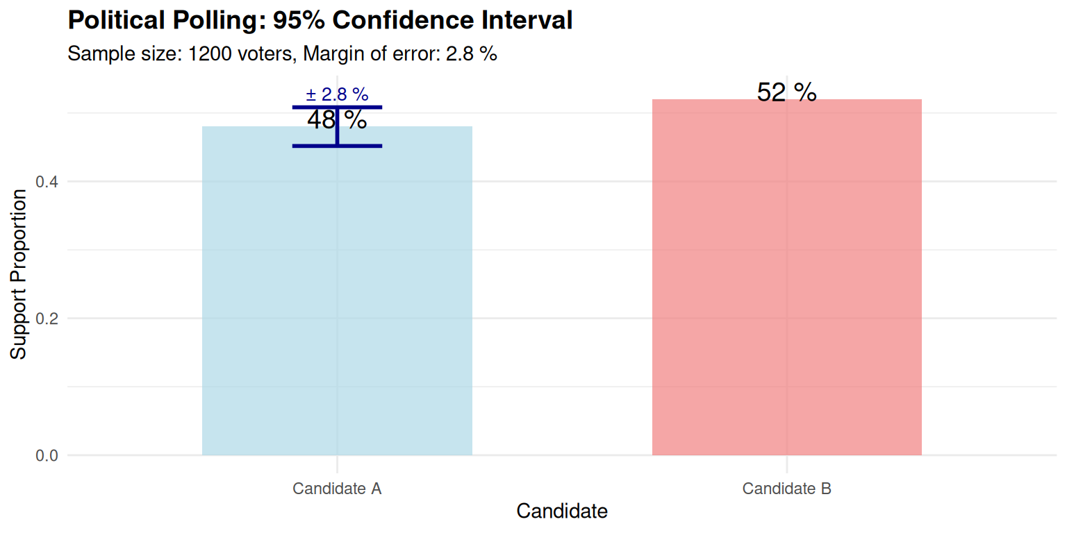
Statistical Analysis:
We’re 95% confident the true support for Candidate A is between 45.2% and 50.8%
Case Study 2: Quality Control Analysis
Context: Manufacturing defect rate monitoring with 500 products, observed defect rate = 2%
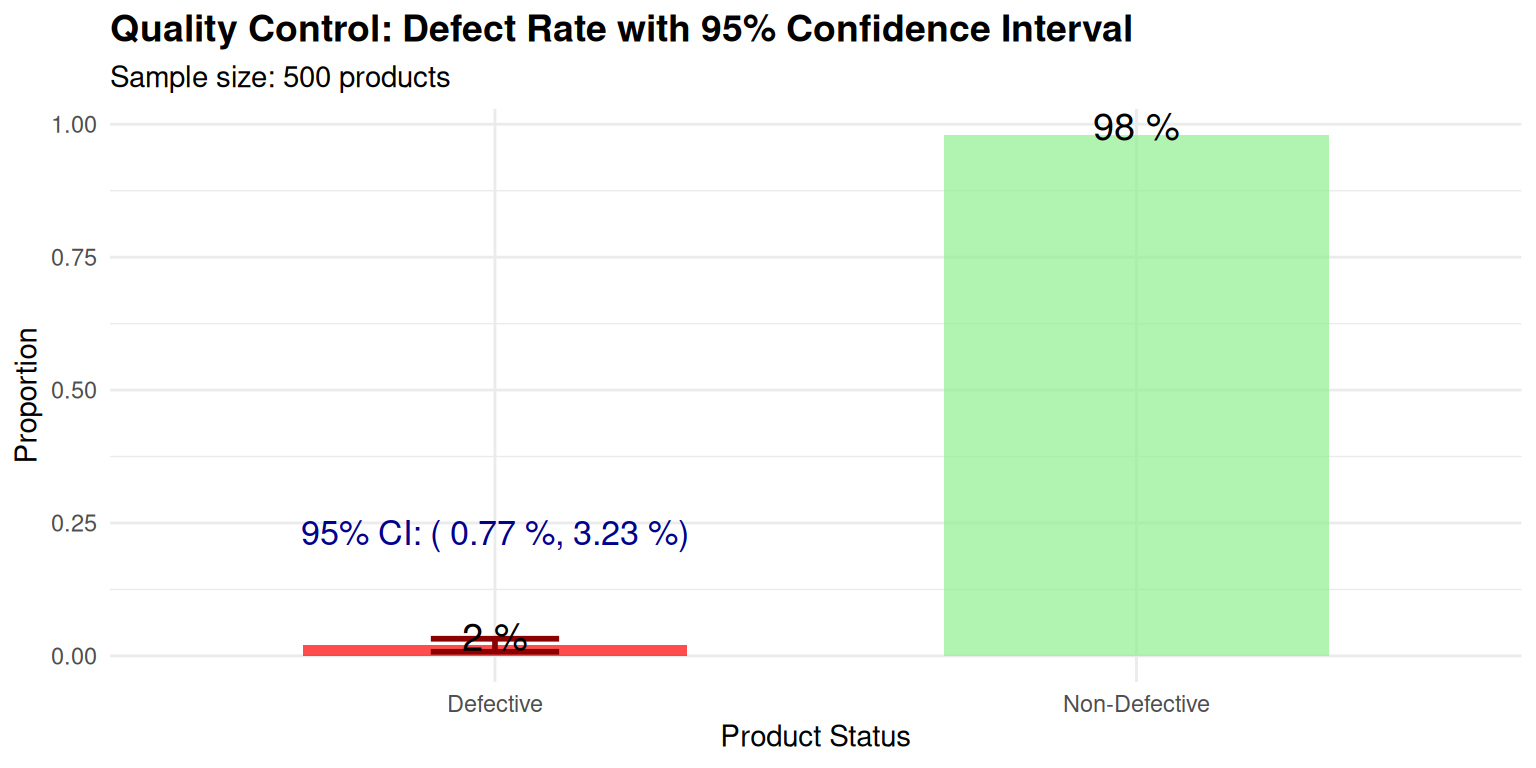
Quality Control Analysis: We’re 95% confident the true defect rate is between 0.8% and 3.2%. If target defect rate is 1%, current process may need improvement
Case Study 3: Medical Research Analysis
Context: Clinical trial for new treatment with 800 patients, success rate = 65%
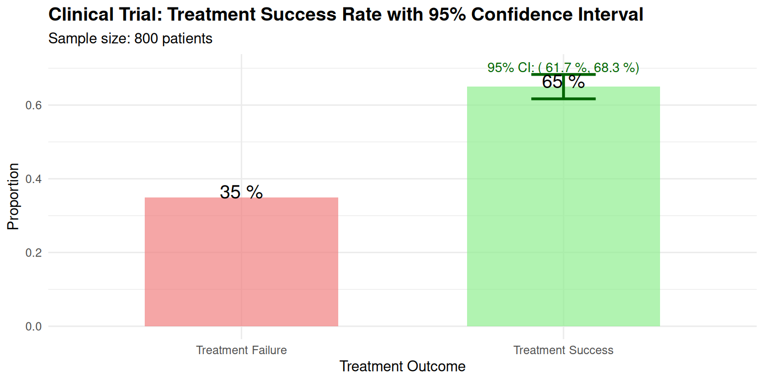
Medical Research Analysis:
We’re 95% confident the true treatment success rate is between 61.7% and 68.3%. The interval provides evidence for treatment effectiveness
Theoretical Formulas
Confidence Interval Calculations
Confidence Interval Formula: \[\text{CI} = \hat{p} \pm z_{\alpha/2} \cdot \sqrt{\frac{\hat{p}(1-\hat{p})}{n}}\]
Margin of Error: \[\text{ME} = z_{\alpha/2} \cdot \sqrt{\frac{\hat{p}(1-\hat{p})}{n}}\]
Sample Size Determination for Proportions
Planning Your Study
Key Question: How large a sample do we need to estimate a proportion with desired precision?
Sample Size Formula: \[n = \left(\frac{z_{\alpha/2}}{ME}\right)^2 \cdot p(1-p)\]
Components:
- \(z_{\alpha/2}\): Critical value for desired confidence level
- \(ME\): Desired margin of error
- \(p\): Estimated proportion (use 0.5 for conservative approach)
Practical Application: This formula helps researchers plan studies with appropriate sample sizes to achieve desired precision!
Confidence Interval Exercises
Practical Exercises Using R
Exercise 1: Basic Confidence Interval Calculation
Sample data: 180 successes out of 400 trials
Calculate 95% CI:
- \(\hat{p} = 180/400 = 0.45\)
- \(SE = \sqrt{0.45 \times 0.55 / 400} = 0.0249\)
- \(95\%\text{ CI} = 0.45 \pm 1.96 \times 0.0249 = (0.401, 0.499)\)
R code:
prop.test(180, 400, conf.level = 0.95)$conf.int
Exercise 2: Sample Size Determination
- Desired margin of error: 3%, estimated proportion: 50%, 95% confidence
- Required sample size: \(n = \left(\frac{1.96}{0.03}\right)^2 \times 0.5 \times 0.5 = 1067.11 \rightarrow 1068\)
- R code:
ceiling((qnorm(0.975)/0.03)^2 * 0.5 * 0.5)
Conservative Sample Size Approach
When p is Unknown
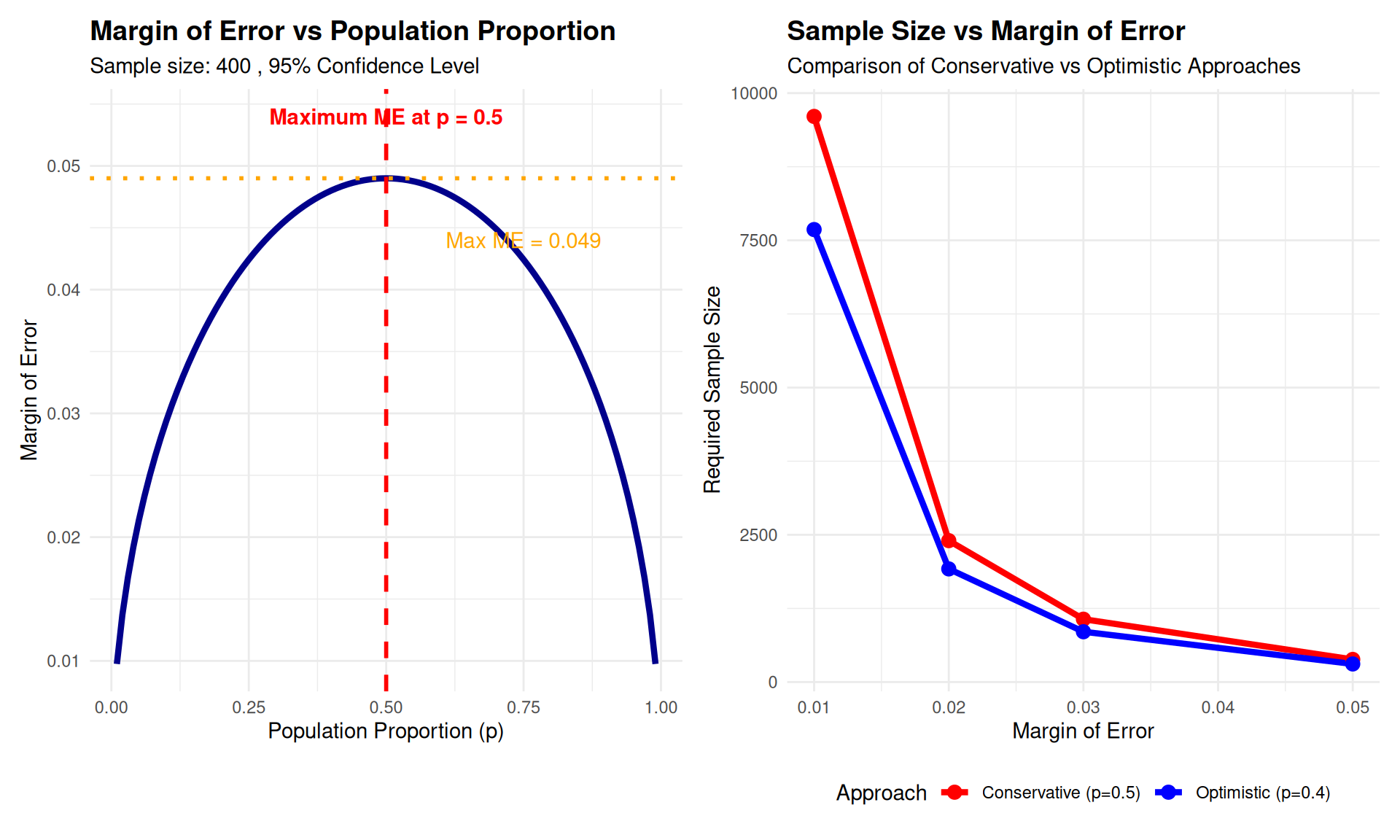
The Conservative Approach: When we have no prior estimate of \(p\), use \(p = 0.5\)
Why 0.5?:
- \(p(1-p)\) reaches its maximum value when \(p = 0.5\)
- This gives the largest possible sample size
- Guarantees desired margin of error regardless of true \(p\)
Conservative Sample Size Formula: \[n = \left(\frac{z_{\alpha/2}}{ME}\right)^2 \cdot 0.25\]
Example: For 95% confidence and 3% margin of error: \[n = \left(\frac{1.96}{0.03}\right)^2 \cdot 0.25 = 1067.11 \rightarrow 1068\]
Key Insight: Conservative approach ensures adequate sample size when prior information is unavailable!
Margin of Error vs Proportion Relationship
Sample Size Calculation Examples
Practical Applications
Example 1: Political Polling
- Desired margin of error: 3%
- Confidence level: 95%
- Conservative approach (p unknown): \[n = \left(\frac{1.96}{0.03}\right)^2 \times 0.25 = 1067.11 \rightarrow 1068\]
- With prior estimate (p = 0.52): \[n = \left(\frac{1.96}{0.03}\right)^2 \times 0.52 \times 0.48 = 1066.05 \rightarrow 1067\]
Example 2: Market Research
- Desired margin of error: 5%
- Confidence level: 90%
- Conservative approach: \[n = \left(\frac{1.645}{0.05}\right)^2 \times 0.25 = 270.6 \rightarrow 271\]
- With prior estimate (p = 0.30): \[n = \left(\frac{1.645}{0.05}\right)^2 \times 0.30 \times 0.70 = 227.4 \rightarrow 228\]
Key Insight: Using prior information can reduce required sample size significantly!
Sample Size Calculation Exercises
Practice Problems
Exercise 5: Basic Sample Size Calculation
- Desired margin of error: 4%
- Confidence level: 95%
- Conservative approach (p unknown)
- Calculate required sample size
Exercise 6: Sample Size with Prior Information
- Desired margin of error: 3%
- Confidence level: 95%
- Prior estimate: p = 0.25
- Calculate required sample size
- Compare with conservative approach
Exercise 7: Impact of Confidence Level
Desired margin of error: 5%
Compare sample sizes for:
- 90% confidence level
- 95% confidence level
- 99% confidence level
Use conservative approach
Exercise 8: Real-World Planning
- Market research firm needs to estimate customer satisfaction
- Desired margin of error: 2%
- Confidence level: 95%
- No prior information available
- Calculate required sample size
- If budget limits sample to 1500, what margin of error can be achieved?
Confidence Interval Exercises
Practical Exercises Using R
Exercise 3: Confidence Level Impact
- Same data: 250 successes out of 500 trials
- 90% CI: \(0.50 \pm 1.645 \times \sqrt{0.5 \times 0.5 / 500} = (0.463, 0.537)\)
- 95% CI: \(0.50 \pm 1.96 \times \sqrt{0.5 \times 0.5 / 500} = (0.456, 0.544)\)
- 99% CI: \(0.50 \pm 2.576 \times \sqrt{0.5 \times 0.5 / 500} = (0.442, 0.558)\)
Exercise 4: Real-World Interpretation
- Market research: 60% prefer new product (95% CI: 55% to 65%, n=400)
- Interpretation: We’re 95% confident the true preference rate is between 55% and 65%
- Business decision: Strong evidence for product launch (interval well above 50%)
Connection with Previous Topics
Building on Statistical Foundations
Relationship to Sampling Distributions (Day 16-18):
- Confidence intervals rely on the sampling distribution properties
- Standard error quantifies the precision of our estimates
- Central Limit Theorem ensures normal approximation for large samples
Relationship to Confidence Intervals for Means (Day 19-20):
- Same conceptual framework: estimate ± margin of error
- Different standard error formulas: \(\sigma/\sqrt{n}\) vs \(\sqrt{p(1-p)/n}\)
- Same critical values from normal/t-distributions
Statistical Continuity:
- All confidence intervals quantify uncertainty in parameter estimation
- The interpretation remains consistent across different parameter types
- The methodology builds systematically from basic principles
Key Statistical Principles
Essential Statistical Concepts:
- Uncertainty Quantification: Confidence intervals provide ranges of plausible values
- Precision Measurement: Standard error quantifies estimation accuracy
- Sample Size Effect: Larger samples → narrower intervals → more precise estimates
- Distribution Independence: CLT works with any population distribution
Statistical Guidelines:
- Success-Failure Condition: Ensure \(n\hat{p} \geq 15\) and \(n(1-\hat{p}) \geq 15\)
- Random Sampling: Essential for valid statistical inference
- Confidence Level: Choose appropriate level for research context
- Interpretation: Focus on the range, not just the point estimate
Next Topic: Applying these principles to hypothesis testing for proportions