Day 26

Math 216: Statistical Thinking

Bastola

Small Sample Inference: Statistical Methods for Limited Data

Key Question: How can we make reliable statistical inferences when sample sizes are small and the Central Limit Theorem doesn’t apply? The t-distribution provides the mathematical framework for valid inference with limited data!

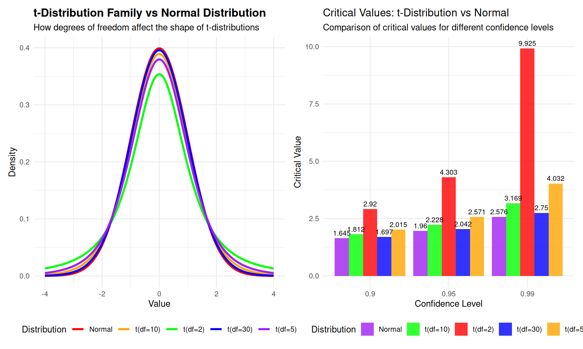
t-Distribution vs Normal Distribution: Small Sample Adaptation

Introduction to Small Sample Confidence Intervals

Background: Confidence intervals and hypothesis testing for large samples (\(n \geq 30\)) rely on the \(z\)-statistic.
Challenge: What happens with a small sample size (\(n < 30\)) where the Central Limit Theorem does not apply?

Adjusting for Small Samples

Population Distribution: If the sample comes from an approximately normal distribution, we can use the \(t\)-statistic.
Standard Deviation: When the population standard deviation \(\sigma\) is unknown and \(n < 30\), using the sample standard deviation \(s\) to approximate \(\sigma\) is unreliable.
Solution: \[ t=\frac{\bar{x}-\mu}{s / \sqrt{n}} \]
- Follows a \(t\)-distribution with degrees of freedom, \(df = n-1\).

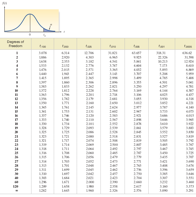
Confidence Interval Using Student’s t-Statistic

When \(\sigma\) is unknown: Use the \(t\)-statistic for confidence intervals.
- For a \(95\%\) confidence interval: \[ \bar{x} \pm t_{\alpha/2} \left(\frac{s}{\sqrt{n}}\right) \] where \(t_{\alpha/2}\) is determined from the \(t\)-distribution table for \(df = n-1\).

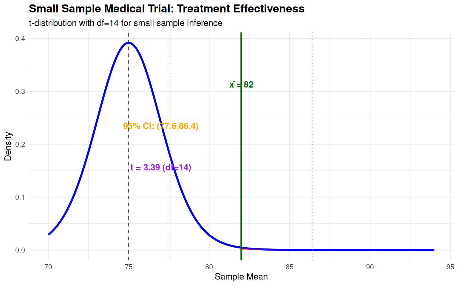
Case Study 1: Medical Research with Small Sample

Context: Clinical trial testing new drug with limited patient availability (n=15)

Statistical Analysis:

Sample Characteristics: n=15, mean=82, SD=8
t-statistic: \(t = \frac{82 - 75}{8/\sqrt{15}} = 3.39\)
95% Confidence Interval: \(82 \pm 2.145 \times (8/\sqrt{15}) = (77.6, 86.4)\)
Interpretation: Strong evidence of treatment effectiveness despite small sample

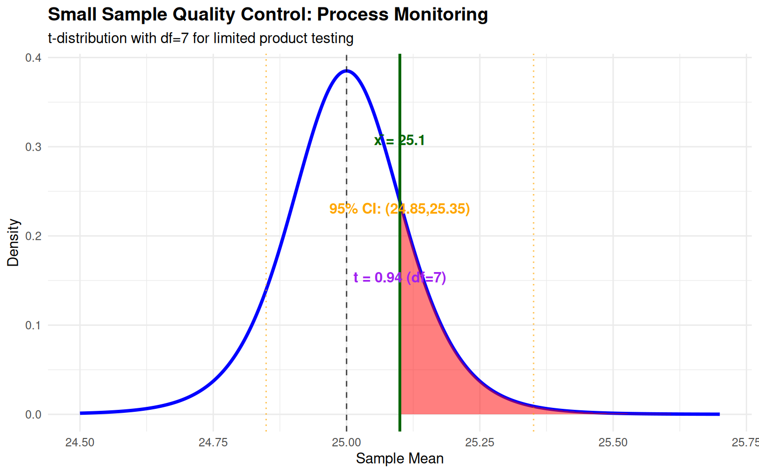
Case Study 2: Quality Control with Limited Data

Context: Manufacturing process testing with expensive products (n=8)

Statistical Analysis:

Sample Characteristics: n=8, mean=25.1, SD=0.3
t-statistic: \(t = \frac{25.1 - 25.0}{0.3/\sqrt{8}} = 0.94\)
95% Confidence Interval: \(25.1 \pm 2.365 \times (0.3/\sqrt{8}) = (24.85, 25.35)\)
Interpretation: No strong evidence of process deviation from target

Formal Hypothesis Testing Notation

General Hypothesis Testing Framework:

Null Hypothesis (\(H_0\)): Statement of no effect or no difference \[H_0: \mu = \mu_0\]
Alternative Hypothesis (\(H_a\)): Statement we want to find evidence for
- Two-tailed test: \(H_a: \mu \neq \mu_0\)
- Right-tailed test: \(H_a: \mu > \mu_0\)
- Left-tailed test: \(H_a: \mu < \mu_0\)
Test Statistic: \[t = \frac{\bar{x} - \mu_0}{s/\sqrt{n}}\] where \(df = n - 1\)
Decision Rule: Reject \(H_0\) if \(|t| > t_{\alpha/2}\) (two-tailed) or \(t > t_\alpha\) (right-tailed) or \(t < -t_\alpha\) (left-tailed)

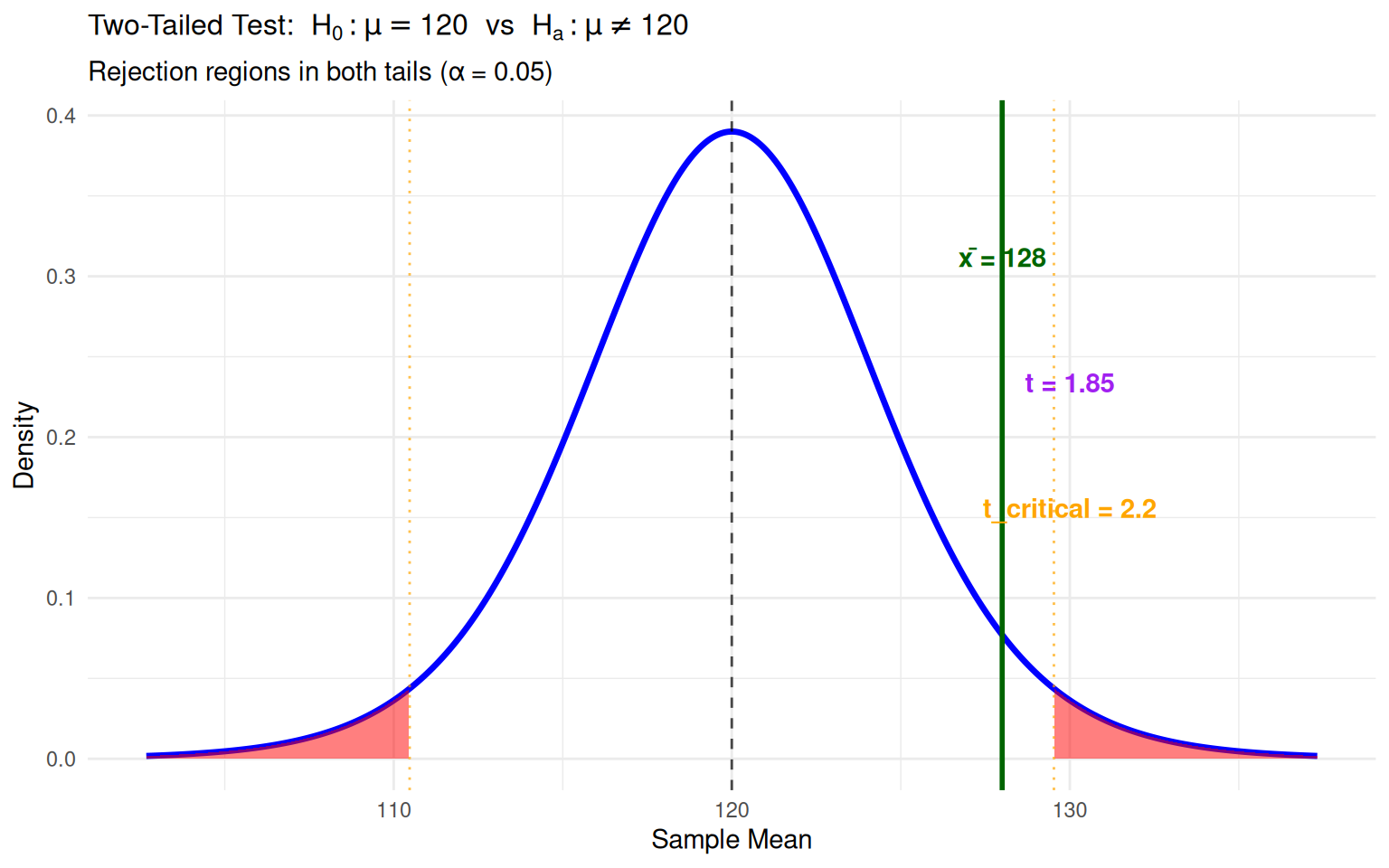
Worked Example 1: Two-Tailed Test

Context: Pharmaceutical company testing if new drug changes blood pressure (n=12)

Interpretation: The observed difference could reasonably occur by chance alone when the null hypothesis is true.

\(H_0\): \(\mu = 120\) mmHg (no change from baseline)
\(H_a\): \(\mu \neq 120\) mmHg (drug changes blood pressure)
Sample: n=12, \(\bar{x} = 128\), s=15
Test Statistic: \[t = \frac{128 - 120}{15/\sqrt{12}} = 1.85\]
Critical Value: \(t_{0.025, 11} = 2.201\)
Decision: Since \(|1.85| < 2.201\), fail to reject \(H_0\)
Conclusion: No significant evidence that drug changes blood pressure

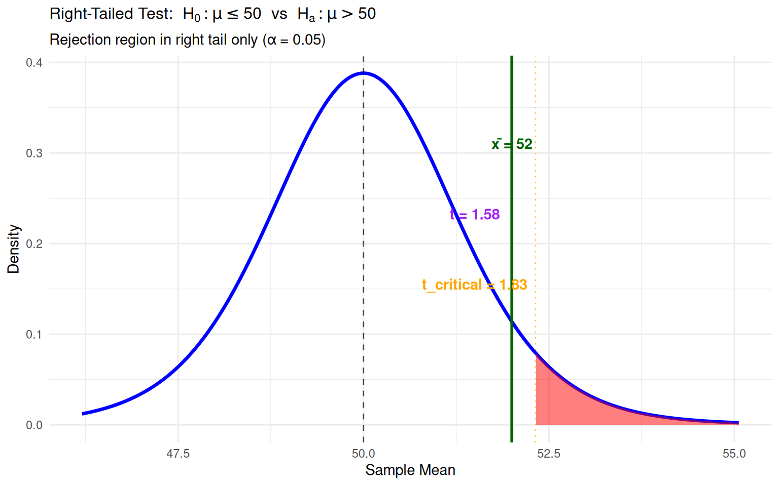
Worked Example 2: Right-Tailed Test

Context: Manufacturing process improvement claim (n=10)

Interpretation: The observed increase in production rate is not statistically significant at the 5% level.

\(H_0\): \(\mu \leq 50\) units/hour (no improvement)
\(H_a\): \(\mu > 50\) units/hour (process improvement)
Sample: n=10, \(\bar{x} = 52\), s=4
Test Statistic: \[t = \frac{52 - 50}{4/\sqrt{10}} = 1.58\]
Critical Value: \(t_{0.05, 9} = 1.833\)
Decision: Since \(1.58 < 1.833\), fail to reject \(H_0\)
Conclusion: No significant evidence of process improvement

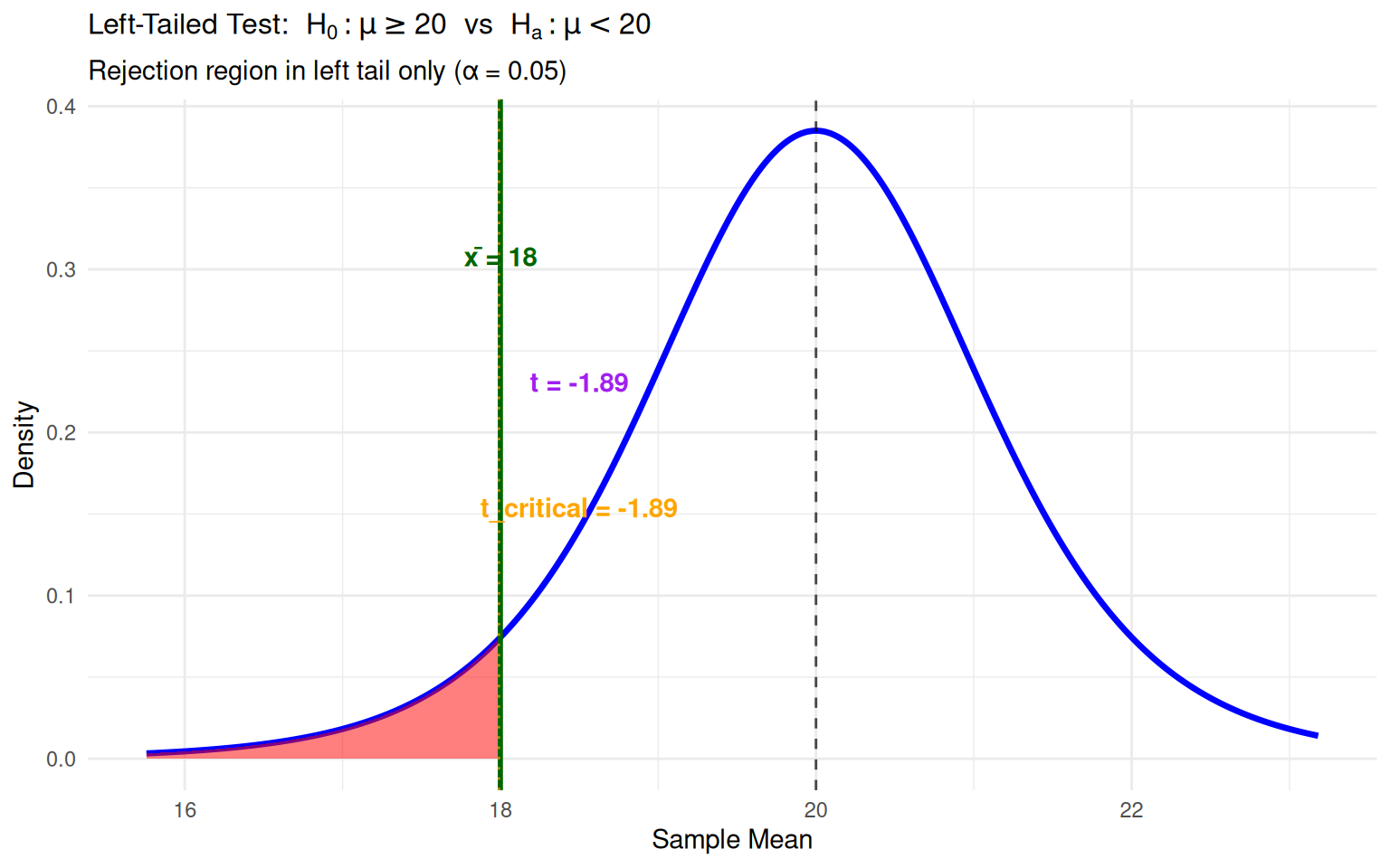
Worked Example 3: Left-Tailed Test

Context: Environmental study testing if pollution levels decreased (n=8)

Interpretation: The observed decrease in pollution levels is not statistically significant at the 5% level.

\(H_0\): \(\mu \geq 20\) ppm (no decrease in pollution)
\(H_a\): \(\mu < 20\) ppm (pollution decreased)
Sample: n=8, \(\bar{x} = 18\), s=3
Test Statistic: \[t = \frac{18 - 20}{3/\sqrt{8}} = -1.89\]
Critical Value: \(t_{0.05, 7} = -1.895\)
Decision: Since \(-1.89 > -1.895\), fail to reject \(H_0\)
Conclusion: No significant evidence of pollution decrease

Summary: Choosing the Right Hypothesis Test

Interpreting Test Results:

Reject \(H_0\): Strong evidence supporting the alternative hypothesis
- Statistical significance ≠ practical importance
- Consider effect size and context
Fail to reject \(H_0\): Insufficient evidence against the null
- Does not prove the null hypothesis is true
- May indicate need for larger sample size

Practical vs Statistical Significance:

Statistical significance: Unlikely result if \(H_0\) is true
Practical significance: Meaningful difference in real-world context
Always consider both when interpreting results

Key Statistical Principles

Essential Small Sample Concepts:

Distribution Adaptation: t-distribution accounts for uncertainty in estimating population SD
Degrees of Freedom: df = n-1 determines t-distribution shape and critical values
Normality Assumption: Population should be approximately normal for small samples
Increased Uncertainty: Smaller samples require wider confidence intervals

Statistical Guidelines:

Sample Size Threshold: Use t-distribution when n < 30 and σ unknown
Normality Check: Verify population normality assumption for small samples
Critical Values: Use t-table or qt() function for appropriate degrees of freedom
Interpretation: Recognize increased uncertainty in small sample results

Common Small Sample Errors

Assumption Violation: Using t-distribution without normality check
Sample Size Misuse: Applying t-distribution to very small samples (n < 5)
Critical Value Errors: Using z-critical values instead of t-critical values
Interpretation Overconfidence: Underestimating uncertainty in small samples