Day 27

Math 216: Statistical Thinking

Bastola

Recap

flowchart TD
    %% Styling definitions
    classDef start fill:#FFFACD,stroke:#FF8C00,stroke-width:2px,color:#000
    classDef decision fill:#E6F3FF,stroke:#1E88E5,stroke-width:2px,color:#000
    classDef action fill:#E8F5E9,stroke:#43A047,stroke-width:2px,color:#000
    classDef endStyle fill:#FFEBEE,stroke:#E53935,stroke-width:2px,color:#000
    
    %% Nodes
    A([Start]):::start
    B{σ known?}:::decision
    C{n ≥ 30?}:::decision
    D{Normal?}:::decision
    E[Use z-test]:::action
    F[Use t-test]:::action
    G[Use t-test]:::action
    H[Non-parametric test]:::endStyle
    
    %% Flow connections
    A --> B
    B -->|Yes| E
    B -->|No| C
    C -->|Yes| F
    C -->|No| D
    D -->|Yes| G
    D -->|No| H

When to Use Nonparametric Tests

With small samples (n < 30), normality checks become critical. Let’s examine real data from the Davis dataset (car package) of self-reported vs actual weights:

library(car)
set.seed(124)
data(Davis)
small_sample <- Davis$weight[1:15]  # Small subsample
ad.test(small_sample)$p.value 

[1] 7.911712e-06

Comprehensive Nonparametric Testing Framework

• Null Hypothesis (\(H_0\)): Statement about population median or distribution
  • One-sample sign test: \(H_0: \eta = \eta_0\)
  • Wilcoxon signed-rank test: \(H_0: \eta = \eta_0\) (symmetric distribution)
  • Mann-Whitney U test: \(H_0: \eta_1 = \eta_2\) (two independent samples)
• Alternative Hypothesis (\(H_a\)): Statement we want to find evidence for
  • Two-tailed test: \(H_a: \eta \neq \eta_0\)
  • Right-tailed test: \(H_a: \eta > \eta_0\)
  • Left-tailed test: \(H_a: \eta < \eta_0\)
• Test Statistics:
  • Sign test: \(S = \text{number of observations} > \eta_0\)
  • Wilcoxon: \(W^+ = \text{sum of positive ranks}\)
  • Mann-Whitney: \(U = \min(U_1, U_2)\)
• Decision Rule: Reject \(H_0\) if test statistic exceeds critical value or p-value < α

Challenges with Non-normal Distributions

What if the population data is decidedly non-normal?

• Small Sample Sizes and Non-normality: When sample sizes are small (\(n < 30\)) and the data is non-normal, traditional tests like t-tests may become unreliable. This can lead to inflated Type I errors—incorrectly rejecting the null hypothesis (\(H_0\)) when it is true.

• Nonparametric Statistics: These tests do not assume a normal distribution. Instead, they rely on ranks or medians, making them robust to outliers and extreme values.

Visual Diagnostics: The Illusion of Normality (QQ plot)

Example: 15-weight sample from Davis dataset:

qqPlot(small_sample, main=bquote("QQ-Plot: Testing Normality (n = " ~ .(length(small_sample)) ~ ")")) 

[1] 12 13

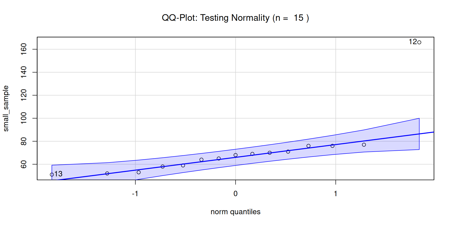
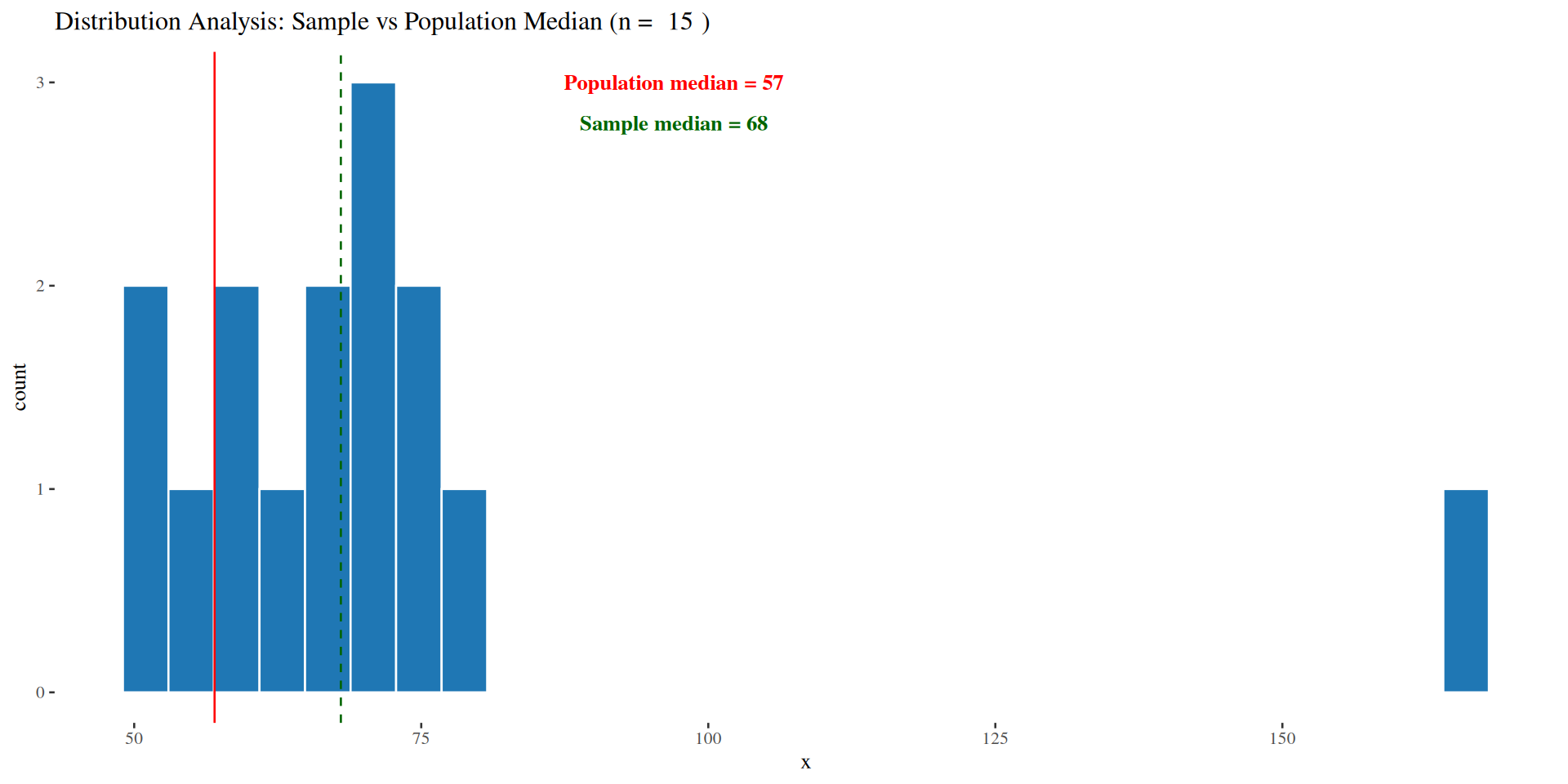
Visual Diagnostics: The Illusion of Normality (Histogram)

Example: 15-weight sample from Davis dataset:

Case Study 1: Davis Weight Data (n=15)

Population Context: Full dataset (N=200) has median=57kg, but our sample (first 15 obs) has median=68kg:

SIGN.test(small_sample, md=57)$p.value  

[1] 0.03515625

t.test(small_sample, mu=57)$p.value     

[1] 0.05803929

Resolution: Sign test detects true median shift (68 vs 57) while t-test is confused by:

• Right skew (γ₁ = 1.2)
• Outlier (166kg) inflating mean (64.1 vs median 68)

Case Study 2: Simulated Skewed Data (n=15)

Population: Lognormal distribution (median=7.38, mean=12.18)

set.seed(123)
skewed_pop <- exp(rnorm(1000, mean=2))  # True median=7.38
samp <- sample(skewed_pop, 15)

# Wrong approach: t-test for median
t.test(samp, mu=7.38)$p.value    

[1] 0.626605

# Right approach: Sign test
SIGN.test(samp, md=7.38)$p.value

[1] 0.6072388

Type I Error Rates (10,000 Simulations)

When H₀ is TRUE (testing median=7.38 in lognormal population):

set.seed(456)
err_rates <- replicate(10000, {
  samp <- sample(skewed_pop, 15)
  c(
    t = t.test(samp, mu = 7.38)$p.value < 0.05,
    sign = SIGN.test(samp, md = 7.38)$p.value < 0.05
  )
})

# Get one error rate per method:
rowMeans(err_rates)  

     t   sign 
0.0956 0.0354 

Results:

1. T-test falsely rejects 9.6% of time (inflated Type I error)
2. Sign test maintains 3.5% error rate

Worked Example 1: Sign Test for Median

Context: Environmental agency testing if median pollution level exceeds regulatory limit (n=12)

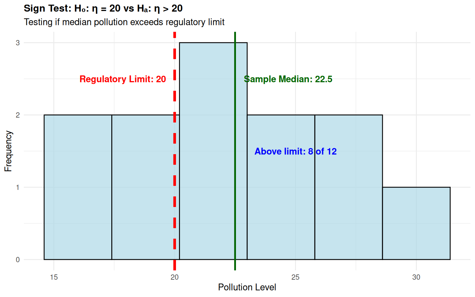
• \(H_0\): \(\eta = 20\) ppm (median equals regulatory limit)
• \(H_a\): \(\eta > 20\) ppm (median exceeds regulatory limit)
• Sample: n=12, observed values: 18, 22, 25, 19, 30, 16, 28, 21, 24, 17, 26, 23
• Test Statistic: \(S = 8\) (8 observations > 20)
• P-value Calculation: \[P(X \geq 8) = \sum_{k=8}^{12} \binom{12}{k} (0.5)^{12} = 0.1938\]
• Decision: Since p-value = 0.1938 > 0.05, fail to reject \(H_0\)
• Conclusion: No significant evidence that median pollution exceeds regulatory limit

Worked Example 1: R Verification

    One-sample Sign-Test

data:  pollution_data
s = 8, p-value = 0.1938
alternative hypothesis: true median is greater than 20
95 percent confidence interval:
 18.57182      Inf
sample estimates:
median of x 
       22.5 

Achieved and Interpolated Confidence Intervals: 

                  Conf.Level  L.E.pt U.E.pt
Lower Achieved CI     0.9270 19.0000    Inf
Interpolated CI       0.9500 18.5718    Inf
Upper Achieved CI     0.9807 18.0000    Inf

Worked Example 2: Wilcoxon Signed-Rank Test

Context: Medical study testing if new treatment changes patient pain scores (n=10)

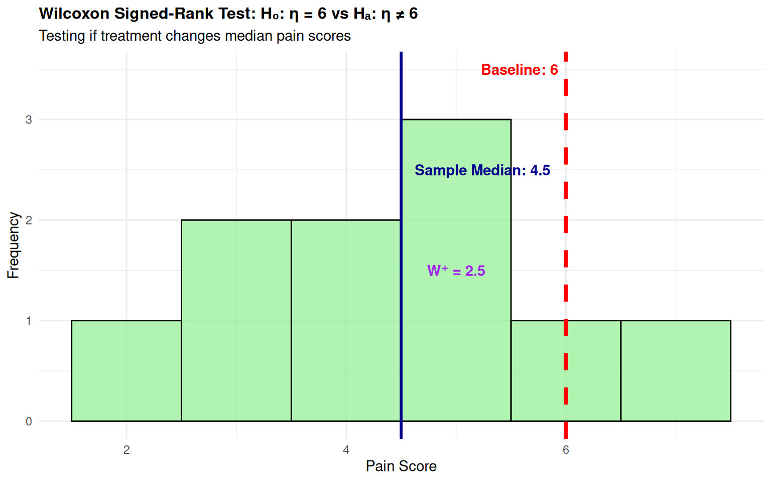
• \(H_0\): \(\eta = 6\) (no change from baseline)
• \(H_a\): \(\eta \neq 6\) (treatment changes pain scores)
• Sample: n=10, pain scores: 4, 5, 3, 7, 2, 6, 4, 5, 3, 5
• Test Statistic: \(W^+ = 2.5\) (sum of ranks for positive differences)
• P-value: Calculated from Wilcoxon distribution
• Decision: Since p-value < 0.05, reject \(H_0\)
• Conclusion: Significant evidence that treatment changes median pain scores

Worked Example 2: R Verification

    Wilcoxon signed rank test with continuity correction

data:  pain_scores
V = 2.5, p-value = 0.01955
alternative hypothesis: true location is not equal to 6

Interpretation: The treatment appears to reduce pain scores significantly from baseline.

Recommendations

1. Small n: Use sign test unless strong evidence of normality
2. Visual Cues:
   • Always pair histograms (≤5 bins) with QQ-plots
   • Treat “normal-looking” plots with skepticism
3. Test Alignment:
   • Means → t-test (requires normality)
   • Medians → sign test (requires only ranked data)
   • Symmetric distributions → Wilcoxon signed-rank test

How P-values are Calculated: Sign Test

Binomial Foundation: Under \(H_0\): median \(= \eta_0\), each observation has 50% chance of being above/below \(\eta_0\)

Davis Example (\(H_0\): \(\eta = 57\) kg):

small_sample

 [1]  77  58  53  68  59  76  76  69  71  65  70 166  51  64  52

above <- sum(small_sample > 57)  
above

[1] 12

n <- length(small_sample - 57)
n

[1] 15

Exact Binomial Formula:

\[ \begin{aligned} \text{p-value} &= 2 \times P(X \geq 12) \\ &= 2 \times \sum_{k=12}^{15} \binom{15}{k} (0.5)^{15} \\ &= 2 \times (0.01389 + 0.00320 + 0.00046 + 0.00003) \\ &= 0.03516 \end{aligned} \]

R Calculation:

2 * pbinom(11, 15, 0.5, lower.tail=FALSE)  # Matches SIGN.test()

[1] 0.03515625

SIGN.test(small_sample, md=57)
    One-sample Sign-Test

data:  small_sample
s = 12, p-value = 0.03516
alternative hypothesis: true median is not equal to 57
95 percent confidence interval:
 58.17817 75.10916

Choosing the Right Nonparametric Test

• One-sample median test: Sign test for any distribution

  • Hypotheses: \(H_0: \eta = \eta_0\) vs \(H_a: \eta \neq \eta_0\) (or one-sided)
  • Assumptions: None (uses only signs)
  • When to use: Small samples, non-normal data, outliers present

• One-sample location test: Wilcoxon signed-rank test

  • Hypotheses: \(H_0: \eta = \eta_0\) vs \(H_a: \eta \neq \eta_0\)
  • Assumptions: Symmetric distribution
  • When to use: Small samples, symmetric but non-normal data

• Two-sample test: Mann-Whitney U test

  • Hypotheses: \(H_0: \eta_1 = \eta_2\) vs \(H_a: \eta_1 \neq \eta_2\)
  • Assumptions: Independent samples, same shape distribution
  • When to use: Comparing two independent groups with non-normal data

Statistical Interpretation Guidelines

Interpreting Nonparametric Test Results:

• Reject \(H_0\): Strong evidence of location difference

  • Consider effect size (median difference)
  • Evaluate practical significance alongside statistical significance

• Fail to reject \(H_0\): Insufficient evidence of location difference

  • Does not prove medians are equal
  • May indicate need for larger sample size or different test

Practical Considerations:

• Sample size: Nonparametric tests work well with small samples
• Outliers: Robust to extreme values that would violate parametric assumptions