Day 28

Math 216: Statistical Thinking

Bastola

Effectiveness of two training programs: Paired Data

Pair	Method A	Method B
1	85	83
2	88	89
3	90	87
4	92	84
5	91	92
6	89	90
7	93	85
8	95	91
9	96	98
10	97	94

Pair	Method A	Method B
11	98	100
12	99	101
13	100	99
14	101	111
15	102	111
16	103	106
17	104	109
18	105	103
19	106	111
20	107	114

Comprehensive Paired t-Test Framework

• Null Hypothesis (\(H_0\)): No difference between paired measurements \[H_0: \mu_d = 0\] where \(\mu_d = \mu_A - \mu_B\) is the population mean difference

• Alternative Hypothesis (\(H_a\)): Statement we want to find evidence for

  • Two-tailed test: \(H_a: \mu_d \neq 0\)
  • Right-tailed test: \(H_a: \mu_d > 0\)
  • Left-tailed test: \(H_a: \mu_d < 0\)

• Test Statistic: \(t = \frac{\bar{d} - \mu_{d0}}{s_d/\sqrt{n}}\) where \(\bar{d} = \frac{\sum d_i}{n}\), \(s_d = \sqrt{\frac{\sum (d_i - \bar{d})^2}{n-1}}\), and \(df = n-1\)

• Decision Rule: Reject \(H_0\) if \(|t| > t_{\alpha/2}\) (two-tailed) or \(t > t_\alpha\) (right-tailed) or \(t < -t_\alpha\) (left-tailed)

Comparing Two Population Means: Paired Difference

Goal: Judge two programs by the within-pair change, \(d_i = A_i - B_i\), canceling out person-to-person noise.
Design: Same participant (or matched pair) supplies both measures; analysis is done on the single column of differences, not the raw scores.

General Testing Procedure

1. Calculate Differences: \(d_i = A_i - B_i\) for each pair

2. Compute Summary Statistics:

   • Mean difference: \(\bar{d} = \frac{\sum d_i}{n}\)
   • Standard deviation: \(s_d = \sqrt{\frac{\sum (d_i - \bar{d})^2}{n-1}}\)

3. Check Conditions:

   • Normality of differences (QQ-plot or Shapiro-Wilk)
   • Random sampling/assignment

4. Select Test Statistic:

   \(t = \frac{\bar{d} - \mu_{d0}}{s_d/\sqrt{n}} \quad \text{with } df = n-1\)

   Where \(\mu_{d0}\) is the hypothesized mean difference (0 under \(H_0\))

5. Make Decision:

   • Compare p-value to \(\alpha\) (typically 0.05)
   • Interpret confidence interval for \(\mu_d\)

Worked Example 1: Right-Tailed Paired t-Test

Context: Medical study testing if new drug increases blood pressure (n=15)

• \(H_0\): \(\mu_d = 0\) (no change in blood pressure)
• \(H_a\): \(\mu_d > 0\) (drug increases blood pressure)
• Sample: n=15 paired measurements
• Test Statistic: \[t = \frac{5.47}{1.30/\sqrt{15}} = 16.26\]
• Critical Value: \(t_{0.05, 14} = 1.761\)
• Decision: Since \(16.26 > 1.761\), reject \(H_0\)
• Conclusion: Strong evidence that drug increases blood pressure

Worked Example 1: R Verification

# Simulated verification
t.test(after, before, paired = TRUE, alternative = "greater")

    Paired t-test

data:  after and before
t = 16.261, df = 14, p-value = 8.705e-11
alternative hypothesis: true mean difference is greater than 0
95 percent confidence interval:
 4.874552      Inf
sample estimates:
mean difference 
       5.466667 

Worked Example 2: Two-Tailed Paired t-Test

Context: Educational study testing if teaching method affects test scores (n=12)

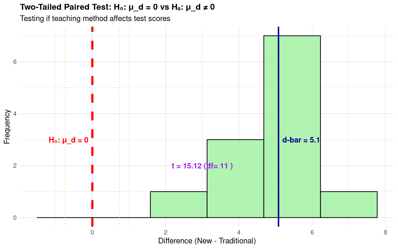
• \(H_0\): \(\mu_d = 0\) (no difference between methods)
• \(H_a\): \(\mu_d \neq 0\) (methods differ)
• Sample: n=12 paired measurements
• Test Statistic: \[t = \frac{5.08}{1.16/\sqrt{12}} = 15.12\]
• Critical Value: \(|t_{0.025, 11}| = 2.201\)
• Decision: Since \(|15.12| > 2.201\), reject \(H_0\)
• Conclusion: Strong evidence that teaching methods differ

Worked Example 2: R Verification

# Simulated verification
t.test(new_method, traditional, paired = TRUE, alternative = "two.sided")

    Paired t-test

data:  new_method and traditional
t = 15.122, df = 11, p-value = 1.047e-08
alternative hypothesis: true mean difference is not equal to 0
95 percent confidence interval:
 4.343445 5.823221
sample estimates:
mean difference 
       5.083333 

Interpretation: The new teaching method appears to significantly improve test scores.

Interpretation Guidance

• Significant Result: Reject \(H_0\) if p-value < \(\alpha\)
  • “Evidence suggests Method A outperforms Method B (t(19)=-0.77, p=0.774)”
• Nonsignificant Result: Fail to reject \(H_0\)
  • “No statistically significant difference detected”
• Always Report:
  • Effect size (mean difference)
  • Confidence interval
  • Practical significance

Selecting Appropriate Statistical Tests

• For Normal Distributions: Apply the paired \(t\)-test.
• For Non-Normal Distributions: Use non-parametric methods that do not assume a normal distribution.

Connection to Confidence Intervals

A 95% CI for \(\mu_d\) is constructed as:

\[\bar{d} \pm t^*_{\alpha/2} \frac{s_d}{\sqrt{n}}\]

• Interpretation: “We are 95% confident the true mean difference lies between [X, Y]”
• Decision Rule: If CI excludes 0, reject \(H_0\) at \(\alpha=0.05\)

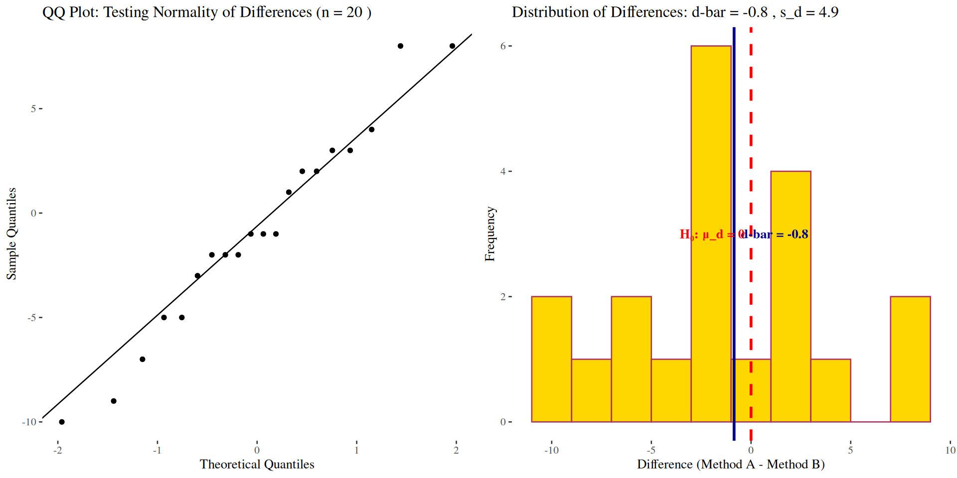
Diagnostic Plots and R Code

• Diagnostic Plots
• R Code

# Define the scores for Method A and Method B
methodA <- c(85, 88, 90, 92, 91, 89, 93, 95, 96, 97, 98,
             99, 100, 101, 102, 103, 104, 105, 106, 107)
methodB <- c(83, 89, 87, 84, 92, 90, 85, 91, 98, 94, 100,
             101, 99, 111, 111, 106, 109, 103, 111, 114)

# Calculate differences
differences <- methodA - methodB

# Generate a QQ plot for normality check
qq_norm <- ggplot(data = tibble(differences), aes(sample = differences)) +
  stat_qq() + stat_qq_line() +
  ggtitle("QQ Plot of Differences")

# Generate a histogram for normality check
histogram <- ggplot(data = as.data.frame(differences), aes(x = differences)) +
  geom_histogram(bins = 10, color = "maroon", fill = "gold") +
  ggtitle("Histogram of Differences")

Preliminary Tests in R

# Perform the Anderson-Darling test for normality
library(nortest)
ad.test(differences)

    Anderson-Darling normality test

data:  differences
A = 0.2269, p-value = 0.787

# Calculate standard deviation of differences
sd(differences) # s_d

[1] 4.92336

# Calculate critical value for t-distribution
qt(0.975, df = 20 - 1) # critical value

[1] 2.093024

t.test for paired samples

# Perform the paired t-test
t.test(methodA, methodB, paired = TRUE, alternative = "greater")

    Paired t-test

data:  methodA and methodB
t = -0.7721, df = 19, p-value = 0.7752
alternative hypothesis: true mean difference is greater than 0
95 percent confidence interval:
 -2.753597       Inf
sample estimates:
mean difference 
          -0.85 

t.test(differences~1, alternative = "greater", data = tibble(differences)) # alternate 1

    One Sample t-test

data:  differences
t = -0.7721, df = 19, p-value = 0.7752
alternative hypothesis: true mean is greater than 0
95 percent confidence interval:
 -2.753597       Inf
sample estimates:
mean of x 
    -0.85