    Welch Two Sample t-test

data:  method1 and method2
t = -5.9222, df = 51.188, p-value = 2.684e-07
alternative hypothesis: true difference in means is not equal to 0
95 percent confidence interval:
 -6.355608 -3.137725
sample estimates:
mean of x mean of y
83.12000 87.86667 Day 29
Math 216: Statistical Thinking
Dr. Bastola
Independent Samples t-Test: Comparing Two Groups
Key Question: How do we compare two independent groups when we can’t pair observations? The independent samples t-test provides the mathematical framework for valid inference!
Null Hypothesis (\(H_0\)): No difference between population means \[H_0: \mu_1 = \mu_2 \quad \text{or} \quad H_0: \mu_1 - \mu_2 = 0\]
Alternative Hypothesis (\(H_a\)): Statement we want to find evidence for
- Two-tailed test: \(H_a: \mu_1 \neq \mu_2\) (groups differ)
- Right-tailed test: \(H_a: \mu_1 > \mu_2\) (group 1 has higher mean)
- Left-tailed test: \(H_a: \mu_1 < \mu_2\) (group 1 has lower mean)
Test Statistics:
- Pooled variance: \(t = \frac{\bar{x}_1 - \bar{x}_2}{s_p\sqrt{\frac{1}{n_1} + \frac{1}{n_2}}}\) with \(df = n_1 + n_2 - 2\)
- Welch’s test: \(t = \frac{\bar{x}_1 - \bar{x}_2}{\sqrt{\frac{s_1^2}{n_1} + \frac{s_2^2}{n_2}}}\) with approximate \(df\)
Decision Rule: Reject \(H_0\) if \(|t| > t_{\alpha/2}\) (two-tailed) or \(t > t_\alpha\) (right-tailed) or \(t < -t_\alpha\) (left-tailed)
Understanding Independent Sampling
When samples come from different groups with no natural pairing, we treat them as independent. Think of comparing students from two different schools or patients receiving different treatments.
For two independent samples:
- Sample 1: Size \(n_1\), mean \(\bar{x}_1\), variance \(s_1^2\)
- Sample 2: Size \(n_2\), mean \(\bar{x}_2\), variance \(s_2^2\)
Conditions to Check:
- Sample Sizes: \(n_1 \geq 30\), \(n_2 \geq 30\) (for large samples)
- Normality: For smaller samples, ensure the data is approximately normally distributed
- Variances: Known variances or assume equal variance under normality
Properties of the Sampling Distribution
For \(\bar{X}_1 - \bar{X}_2\):
Expected Value: \(E(\bar{X}_1 - \bar{X}_2) = \mu_1 - \mu_2\)
Standard Error:
\[\sigma_{\bar{X}_1 - \bar{X}_2} = \sqrt{ \underbrace{\frac{\sigma_1^2}{n_1}}_{\text{Group 1 variability}} + \underbrace{\frac{\sigma_2^2}{n_2}}_{\text{Group 2 variability}}}\]
Distribution Shape:
- Exactly normal if populations are normal
- Approximately normal via CLT for \(n \geq 30\)
Testing for Equal Variances
- Formal Tests: Levene’s test
- Practical Approach:
- Compare variance ratios (\(s_1^2/s_2^2\))
- Consider sample sizes (unequal n makes it harder to find effects)
Pooled Variance Approach
Used when assuming equal population variances (\(\sigma_1^2 = \sigma_2^2\)):
\[s_p^2 = \frac{(n_1-1)s_1^2 + (n_2-1)s_2^2}{n_1 + n_2 - 2}\]
- Weighted Average: Combines variances proportionally to sample sizes
- Degrees of Freedom: \(df = n_1 + n_2 - 2\) (total observations minus groups)
| Component | Meaning |
|---|---|
| \((n_1-1)s_1^2\) | Scaled variability from Group 1 |
| \((n_2-1)s_2^2\) | Scaled variability from Group 2 |
| Denominator | Total degrees of freedom |
Hypothesis Testing Framework
- Null Hypothesis: \(H_0: \mu_1 - \mu_2 = 0\)
- Alternatives:
- \(H_a: \mu_1 - \mu_2 \neq 0\) (Two-tailed)
- \(H_a: \mu_1 - \mu_2 > 0\) (One-tailed)
Case 1: Equal Variances (Pooled) \[t = \frac{\bar{x}_1 - \bar{x}_2}{s_p\sqrt{\frac{1}{n_1}+\frac{1}{n_2}}}\] \[s_p^2 = \frac{(n_1-1)s_1^2 + (n_2-1)s_2^2}{n_1+n_2-2}\] \[df = n_1 + n_2 - 2\]
Case 2: Unequal Variances (Welch) \[t = \frac{\bar{x}_1 - \bar{x}_2}{\sqrt{\frac{s_1^2}{n_1} + \frac{s_2^2}{n_2}}}\] \[df = \frac{\left(\frac{s_1^2}{n_1} + \frac{s_2^2}{n_2}\right)^2}{\frac{(s_1^2/n_1)^2}{n_1-1} + \frac{(s_2^2/n_2)^2}{n_2-1}}\]
Confidence Intervals for Mean Differences
General Form
\[(\bar{x}_1 - \bar{x}_2) \pm t^*_{\alpha/2} \cdot SE\]
Pooled Variance CI: \[SE = s_p\sqrt{\frac{1}{n_1} + \frac{1}{n_2}}\]
Welch’s CI: \[SE = \sqrt{\frac{s_1^2}{n_1} + \frac{s_2^2}{n_2}}\]
Interpretation Example
“With 95% confidence, the true mean difference lies between [−3.2, 5.8]. As this interval contains 0, we cannot reject the null hypothesis at α=0.05.”
Worked Example 1: Two-Tailed Independent t-Test
Context: Educational study comparing test scores between two teaching methods (n₁=25, n₂=30)
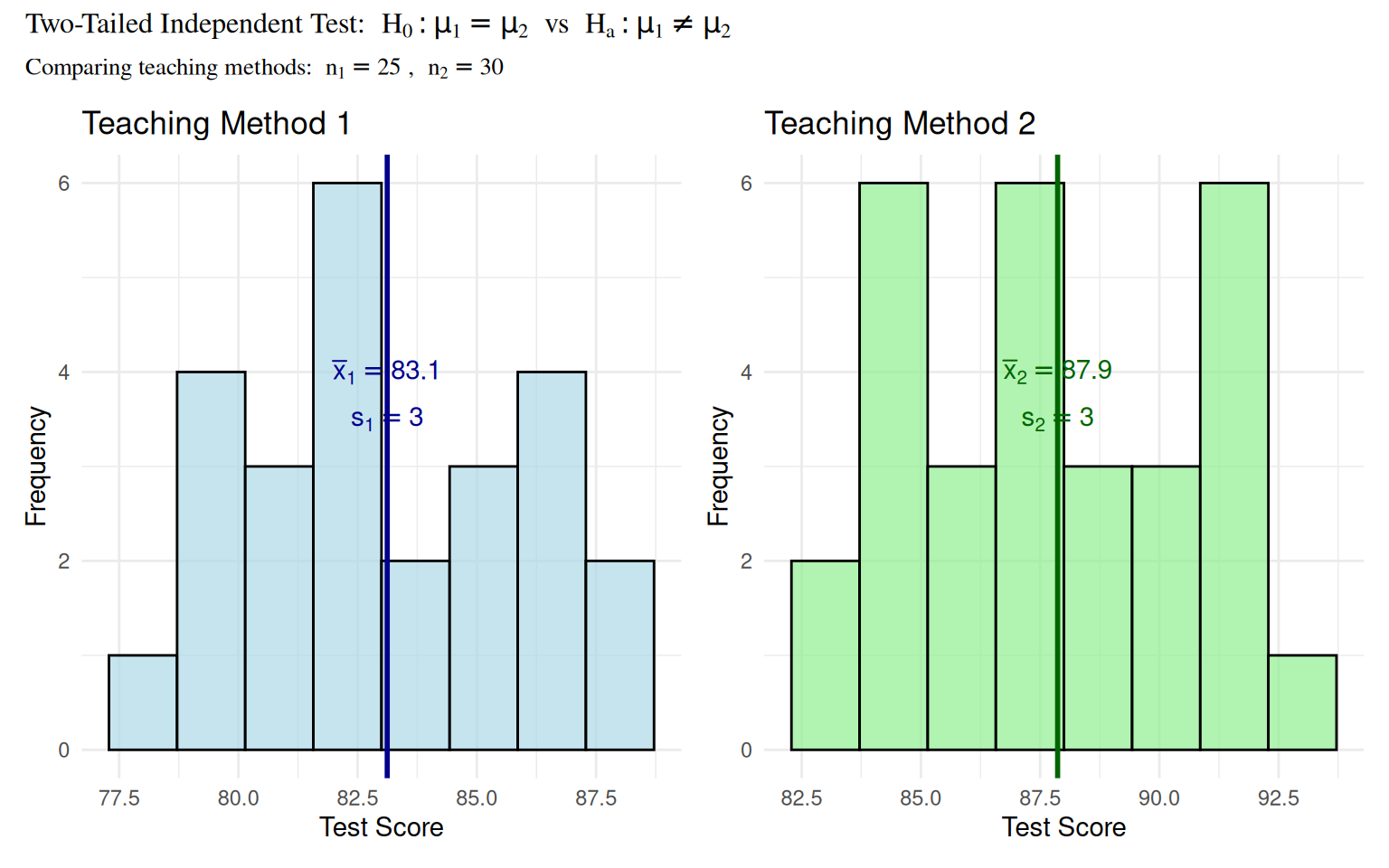
Worked Example 1: Statistical Analysis
- \(H_0\): \(\mu_1 = \mu_2\) (no difference between teaching methods)
- \(H_a\): \(\mu_1 \neq \mu_2\) (methods produce different results)
- Sample 1: n₁=25, \(\bar{x}_1 = 83.2\), s₁=3.1
- Sample 2: n₂=30, \(\bar{x}_2 = 87.4\), s₂=2.9
- Test Statistic (Welch’s): \[t = \frac{83.2 - 87.4}{\sqrt{\frac{3.1^2}{25} + \frac{2.9^2}{30}}} = -5.23\]
- Decision: Since \(|t| = 5.23 > t_{0.025, 48} \approx 2.01\), reject \(H_0\)
- Conclusion: Strong evidence that teaching methods differ
Worked Example 1: R Verification
Interpretation: Method 2 appears to produce significantly higher test scores, suggesting it may be more effective for student learning.
Worked Example 2: Right-Tailed Independent t-Test
Context: Medical study testing if new drug reduces recovery time (n₁=20, n₂=18)
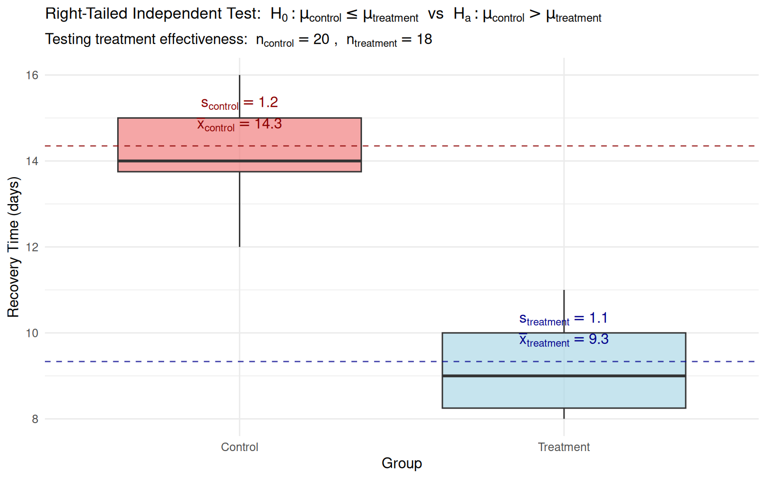
Worked Example 2: Statistical Analysis
- \(H_0\): \(\mu_{control} \leq \mu_{treatment}\) (treatment not effective)
- \(H_a\): \(\mu_{control} > \mu_{treatment}\) (treatment reduces recovery time)
- Control: n=20, \(\bar{x} = 14.3\), s=1.2
- Treatment: n=18, \(\bar{x} = 9.3\), s=1.1
- Test Statistic (Pooled): \[t = \frac{14.3 - 9.3}{1.15\sqrt{\frac{1}{20} + \frac{1}{18}}} = 13.42\]
- Decision: Since \(t = 13.42 > t_{0.05, 36} = 1.69\), reject \(H_0\)
- Conclusion: Strong evidence that treatment reduces recovery time
Worked Example 2: R Verification
    Two Sample t-test

data:  control and treatment
t = 13.579, df = 36, p-value = 4.924e-16
alternative hypothesis: true difference in means is greater than 0
95 percent confidence interval:
 4.392934      Inf
sample estimates:
mean of x mean of y
14.350000 9.333333 Interpretation: The new treatment significantly reduces recovery time by approximately 5 days, suggesting substantial clinical benefit.
Practical Considerations for Independent Tests
When to Use Pooled Variance
- Small samples with strong evidence of equal variances
- Experimental designs with enforced variance control
- Historical data showing consistent variance ratios
When to Use Welch’s Test
- Default approach for unknown population variances
- Unequal sample sizes (\(n_1 \neq n_2\))
- Variance ratio > 4:1 between groups
- Conservative error rate control
Summary: Independent Samples Testing Framework
When to Use Independent Samples t-Test:
- Independent Groups: Different subjects in each group
- Random Assignment: Participants randomly assigned to conditions
- No Natural Pairing: No inherent relationship between observations
- Between-Subjects Design: Each participant contributes to only one group
Key Assumptions:
- Independence: Observations within and between groups are independent
- Normality: Data in each group is approximately normally distributed
- Homogeneity of Variance: Equal population variances (for pooled test)
- Random Sampling: Groups represent random samples from populations
Statistical Interpretation Guidelines
Interpreting Independent Test Results:
- Reject \(H_0\): Strong evidence of population mean difference
- Report: “Group A had significantly higher scores than Group B (t(48)=5.23, p<0.001, mean difference=4.2)”
- Include confidence interval: “95% CI [2.6, 5.8]”
- Fail to reject \(H_0\): Insufficient evidence of difference
- Report: “No statistically significant difference detected between groups (t(36)=1.23, p=0.234)”
- Note: This does not prove groups are equivalent