flowchart LR
    %% Styling definitions
    classDef start fill:#FFFACD,stroke:#FF8C00,stroke-width:2px,color:#000
    classDef decision fill:#E6F3FF,stroke:#1E88E5,stroke-width:2px,color:#000
    classDef action fill:#E8F5E9,stroke:#43A047,stroke-width:2px,color:#000
    classDef endStyle fill:#FFEBEE,stroke:#E53935,stroke-width:2px,color:#000

    %% Nodes
    A([Start]):::start
    B{σ known?}:::decision
    C{n ≥ 30?}:::decision
    D{Normal?}:::decision
    E[Use z-test]:::action
    F[Use t-test]:::action
    G[Use t-test]:::action
    H[Use non-parametric test<br/>Sign/Wilcoxon]:::endStyle

    %% Flow connections
    A --> B
    B -->|Yes| E
    B -->|No| C
    C -->|Yes| F
    C -->|No| D
    D -->|Yes| G
    D -->|No| H
Day 30
Math 216: Statistical Thinking
Bastola
Statistical Test: Choosing the Right Tool
Key Question: How do we choose the right statistical test for our data? The answer lies in understanding your research question and data characteristics!
One-Sample vs Two-Sample Tests
One-Sample Tests: When comparing a sample to a known population value
- \(H_0\): \(\mu = \mu_0\) or \(\eta = \eta_0\)
- Parametric: z-test (\(\sigma\) known), t-test (\(\sigma\) unknown)
- Nonparametric: Sign test, Wilcoxon signed-rank test
Two-Sample Tests: When comparing two different groups
- \(H_0\): \(\mu_1 = \mu_2\) or \(\eta_1 = \eta_2\)
- Independent: t-test (pooled/Welch), Mann-Whitney U test
- Paired: Paired t-test, Wilcoxon signed-rank test
What Really Matters
When selecting a statistical test, consider these critical factors:
Data Type: Continuous, ordinal, or categorical?
Distribution: Normal, non-normal, or unknown shape?
Sample Size: Large (\(n >= 30\)) or small (\(n < 30\))?
Variance: Known, unknown, equal, or unequal?
Design: Independent, paired, or repeated measures?
Key Principle:
Match your test to your data characteristics and research question!
One Sample Tests Summary
Two Samples Tests Summary
flowchart LR
    %% Styling definitions
    classDef start fill:#FFFACD,stroke:#FF8C00,stroke-width:2px,color:#000
    classDef decision fill:#E6F3FF,stroke:#1E88E5,stroke-width:2px,color:#000
    classDef action fill:#E8F5E9,stroke:#43A047,stroke-width:2px,color:#000
    classDef endStyle fill:#FFEBEE,stroke:#E53935,stroke-width:2px,color:#000

    %% Nodes
    A([Two Samples]):::start
    B{Paired data?}:::decision
    C{σ known?}:::decision
    E{n ≥ 30?}:::decision
    F{Normal both?}:::decision
    G[Use z-test]:::action
    H[Use paired t-test]:::action
    I[Use t-test]:::action
    J[Use t-test]:::action
    K[Use Mann-Whitney U<br/>Wilcoxon rank-sum]:::endStyle

    %% Flow connections
    A --> B
    B -->|Yes| H
    B -->|No| C
    C -->|Yes| G
    C -->|No| E
    E -->|Yes| I
    E -->|No| F
    F -->|Yes| J
    F -->|No| K
Wilcoxon Test in R
One-Sample Wilcoxon Signed Rank Test
Non-parametric test of whether a single sample’s median differs from a hypothesized value.
Paired Wilcoxon Signed Rank Test
Tests median differences between paired measurements (non-parametric alternative to paired t-test).
Wilcoxon Rank Sum/Mann-Whitney U Test
Non-parametric comparison of two independent sample distributions (location).
Parametric Tests in R
z-Test (Known σ²)
Requires BSDA package. For known population variance:
Student’s t-Test
Compare means (one-sample, two-sample, or paired). Default assumes unequal variances:
Summary Statistics Tests (BSDA)
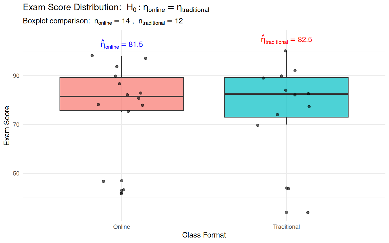
Analysis of Exam Scores: Online vs Traditional Classroom
Real Educational Question: Do students perform differently in online vs traditional classroom settings?
Online Class Data (n₁=14)
Scores: 78, 82, 83, 87, 75, 43, 78, 42, 94, 47, 98, 90, 97, 81
Traditional Class Data (n₂=12)
Scores: 83, 82, 92, 100, 74, 90, 44, 84, 77, 89, 70, 34
| Class_Type | n | Median |
|---|---|---|
| Online | 14 | 81.5 |
| Traditional | 12 | 82.5 |
Statistical Challenge & Method Choice
The Statistical Challenge: Small samples with potential non-normality and outliers - perfect scenario for non-parametric methods!
Why We Choose Mann-Whitney U Test:
- Independent samples (different students in each format)
- Small sample sizes (n₁=14, n₂=12)
- Potential outliers and non-normal distributions
- Compare location parameters without strict assumptions
Mann-Whitney U Test Approach
Our Statistical Approach: We’ll use the Mann-Whitney U test (also called Wilcoxon rank-sum test), which lets us compare two independent samples without worrying about normality assumptions!
Setting Up Our Hypotheses
Formal Hypotheses:
- Null Hypothesis (\(H_0\)): No real difference in population medians
\[H_0: \eta_{online} = \eta_{traditional}\]
- Alternative Hypothesis (\(H_a\)): Two-tailed test for any difference
\[H_a: \eta_{online} \neq \eta_{traditional}\]
Test Parameters and Assumptions
Test Parameters:
- Significance Level: \(\alpha = 0.05\) (our standard threshold)
- Test Type: Two-tailed Mann-Whitney U test
- Sample Sizes: n₁=14 (online), n₂=12 (traditional)
- Test Statistic: U = min(U₁, U₂)
What We’re Assuming:
- Independence: Students in each group are independent
- Ordinal Scale: Exam scores can be meaningfully ranked
- Same Shape: Distributions have similar shape (location shift alternative)
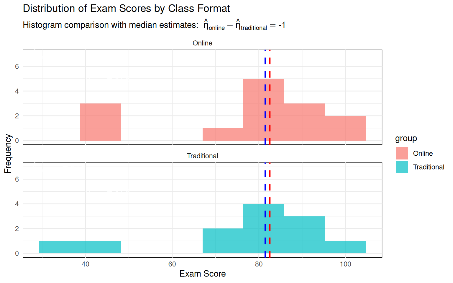
Data Visualization: Explore Distributions
Histogram Comparison
Running the Mann-Whitney U Test
Mann-Whitney U Test Results:Test Statistic (W) = 85.5 P-value = 0.9589513 Alternative Hypothesis: two.sided Decision: Fail to reject H₀ (p ≥ 0.05)
Conclusion: No significant evidence of difference in median exam scoresMann-Whitney U Outcome & Justification
- W = 85.5, p = 0.959 → Retain H₀ (α = 0.05)
- Medians: online 81.5 vs. traditional 82.5 (negligible gap)
- Interpretation: Format does not shift median exam score
- Why this test? Non-normal data, outliers, small n, ordinal scores—rank-based & robust
- Next step: look beyond p-values to pedagogy & learner context
Test Selection by Data
Data Characteristics:
Data Type Considerations
- Continuous vs Categorical: Scale of measurement
- Normal vs Non-normal: Distribution shape
- Large vs Small: Sample size (n ≥ 30 vs n < 30)
Parameter of Interest:
- Means: Parametric tests (t-tests, z-tests)
- Medians: Nonparametric tests (sign, Wilcoxon)
Practical Test Guidelines
Large samples (n ≥ 30):
- Use z-tests when population variance known
- Use t-tests when population variance unknown
- CLT provides approximate normality
Small samples (n < 30):
- Check normality assumption carefully
- Use t-tests if population approximately normal
- Use nonparametric tests if non-normal or outliers
Your R Toolkit
Parametric Tests
t.test(x, mu = μ₀)                    # One-sample t-test
t.test(x, y)                          # Two-sample t-test
t.test(x, y, paired = TRUE)           # Paired t-test
Nonparametric Tests
wilcox.test(x, mu = η₀)              # One-sample Wilcoxon
wilcox.test(x, y)                    # Mann-Whitney U test
wilcox.test(x, y, paired = TRUE)     # Paired Wilcoxon