Day 31

Math 216: Statistical Thinking

Bastola

Proportion Inference Framework

Statistical Continuity: Building on previous inference methods

  • Days 19-24: Large sample inference for population means
  • Days 26-30: Small sample and nonparametric methods
  • Day 31: Extending inference to categorical data via proportions

Key Conceptual Shift:

  • Continuous Data: Means and medians (quantitative variables)
  • Categorical Data: Proportions and percentages (qualitative variables)
  • Common Framework: Both use sampling distribution theory and CLT

Formal Hypothesis Testing for Proportions

Null Hypothesis (\(H_0\)): Statement about population proportion \[H_0: p = p_0\]

Alternative Hypothesis (\(H_a\)): Statement we want to find evidence for

  • Two-tailed test: \(H_a: p \neq p_0\)
  • Right-tailed test: \(H_a: p > p_0\)
  • Left-tailed test: \(H_a: p < p_0\)

Test Statistic: \[z = \frac{\hat{p} - p_0}{\sqrt{\frac{p_0(1-p_0)}{n}}}\]

Decision Rule: Reject \(H_0\) if \(|z| > z_{\alpha/2}\) (two-tailed) or \(z > z_\alpha\) (right-tailed) or \(z < -z_\alpha\) (left-tailed)

Hypothesis Formulations

Alternative Hypothesis (\(H_a\)): Statement we want to find evidence for

  • Two-tailed test: \(H_a: p \neq p_0\)
  • Right-tailed test: \(H_a: p > p_0\)
  • Left-tailed test: \(H_a: p < p_0\)

Decision Rules:

  • Two-tailed: Reject \(H_0\) if \(|z| > z_{\frac{\alpha}{2}}\)
  • Right-tailed: Reject \(H_0\) if \(z > z_{\alpha}\)
  • Left-tailed: Reject \(H_0\) if \(z < -z_{\alpha}\)

Sampling Distribution Structure

Definition: Sample proportion \(\hat{p} = \frac{X}{n}\) where \(X \sim \text{Binomial}(n, p)\)

Exact Properties:

  1. Expected Value: \(E(\hat{p}) = p\)
  2. Variance: \(\text{Var}(\hat{p}) = \frac{p(1-p)}{n}\)
  3. Standard Error: \(\sigma_{\hat{p}} = \sqrt{\frac{p(1-p)}{n}}\)

Large Sample Approximation: - Central Limit Theorem for Proportions: \[\hat{p} \stackrel{\text{approx}}{\sim} N\left(p, \sqrt{\frac{p(1-p)}{n}}\right)\] - Conditions for Normality: \[np \geq 15 \quad \text{and} \quad n(1-p) \geq 15\]

Two-Tailed Poll Example Part 1

Context: Political polling to test if candidate support differs from historical baseline (n=400)

Two-Tailed Poll Example: Steps

  • \(H_0\): \(p = 0.50\) (candidate support equals historical baseline)
  • \(H_a\): \(p \neq 0.50\) (candidate support differs from baseline)
  • Sample: \(n=400\), \(\hat{p} = 0.48\)
  • Test Statistic: \[z = \frac{\hat{p} - p_0}{\sqrt{\frac{p_0(1-p_0)}{n}}} = \frac{0.48 - 0.50}{\sqrt{\frac{0.50(1-0.50)}{400}}} = -0.80\]
  • Critical Value: \(z_{\alpha/2} = z_{0.025} = 1.96\)
  • Decision: Since \(|z| = |-0.80| < 1.96\), fail to reject \(H_0\)
  • Conclusion: No significant evidence that candidate support differs from historical baseline

Two-Tailed Poll Example Part 1: R Verification

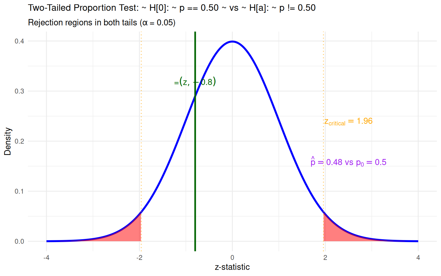
# Two-tailed proportion test
prop.test(x = 192, n = 400, p = 0.50, alternative = "two.sided", correct = FALSE)

    1-sample proportions test without continuity correction

data:  192 out of 400
X-squared = 0.64, df = 1, p-value = 0.4237
alternative hypothesis: true p is not equal to 0.5
95 percent confidence interval:
 0.4314634 0.5289171
sample estimates:
   p 
0.48 

Interpretation: The observed difference in candidate support could reasonably occur by chance alone.

Worked Example 2: Right-Tailed Proportion Test

Context: Quality control testing if new manufacturing process reduces defect rate (n=500)

Worked Example 2: Formal Hypothesis Test

  • \(H_0\): \(p \geq 0.10\) (defect rate not improved)
  • \(H_a\): \(p < 0.10\) (defect rate reduced)
  • Sample: \(n=500\), \(\hat{p} = 0.08\)
  • Test Statistic: \[z = \frac{\hat{p} - p_0}{\sqrt{\frac{p_0(1-p_0)}{n}}} = \frac{0.08 - 0.10}{\sqrt{\frac{0.10(1-0.10)}{500}}} = -1.49\]
  • Critical Value: \(z_{\alpha} = z_{0.05} = -1.645\)
  • Decision: Since \(z = -1.49 > -1.645\), fail to reject \(H_0\)
  • Conclusion: No significant evidence that new process reduces defect rate

Worked Example 2: R Verification

# Right-tailed proportion test
prop.test(x = 40, n = 500, p = 0.10, alternative = "less", correct = FALSE)

    1-sample proportions test without continuity correction

data:  40 out of 500
X-squared = 2.2222, df = 1, p-value = 0.06802
alternative hypothesis: true p is less than 0.1
95 percent confidence interval:
 0.000000 0.102291
sample estimates:
   p 
0.08 

Interpretation: While defect rate appears lower, the evidence is not statistically significant at α=0.05.