flowchart TD
    %% Styling definitions
    classDef start fill:#FFFACD,stroke:#FF8C00,stroke-width:2px,color:#000
    classDef decision fill:#E6F3FF,stroke:#1E88E5,stroke-width:2px,color:#000
    classDef correct fill:#E8F5E9,stroke:#43A047,stroke-width:2px,color:#000
    classDef error fill:#FFEBEE,stroke:#E53935,stroke-width:2px,color:#000

    %% Nodes
    A([Start: Hypothesis Test]):::start
    B{Reject H₀?}:::decision
    C{H₀ True?}:::decision
    D[Correct Decision<br/>True Negative<br/>1-α]:::correct
    E[Type II Error<br/>False Negative<br/>β]:::error
    F[Type I Error<br/>False Positive<br/>α]:::error
    G[Correct Decision<br/>True Positive<br/>1-β]:::correct

    %% Flow connections
    A --> B
    B -->|No| C
    B -->|Yes| C
    C -->|Yes| D
    C -->|No| E
    C -->|Yes| F
    C -->|No| G
Day 32
Math 216: Statistical Thinking
Bastola
How Statistical Decisions Can Go Wrong
Key Question: What happens when our statistical conclusions are wrong? Understanding Type I and Type II errors helps us make better decisions and design more effective studies!
The Two Types of Statistical Mistakes:
Type I Error (\(\alpha\)): False alarm! Rejecting \(H_0\) when it’s actually true \[\alpha = P(\text{Reject } H_0 \mid H_0 \text{ true})\]
Type II Error (\(\beta\)): Missed opportunity! Failing to reject \(H_0\) when \(H_a\) is true \[\beta(\mu) = P(\text{Fail to reject } H_0 \mid \mu = \mu_a)\]
Power (\(1-\beta\)): Getting it right! Correctly detecting real effects \[\text{Power}(\mu) = 1 - \beta(\mu) = P(\text{Reject } H_0 \mid \mu = \mu_a)\]
Hypothesis Testing Errors
Real-World Example: Quality Control Testing
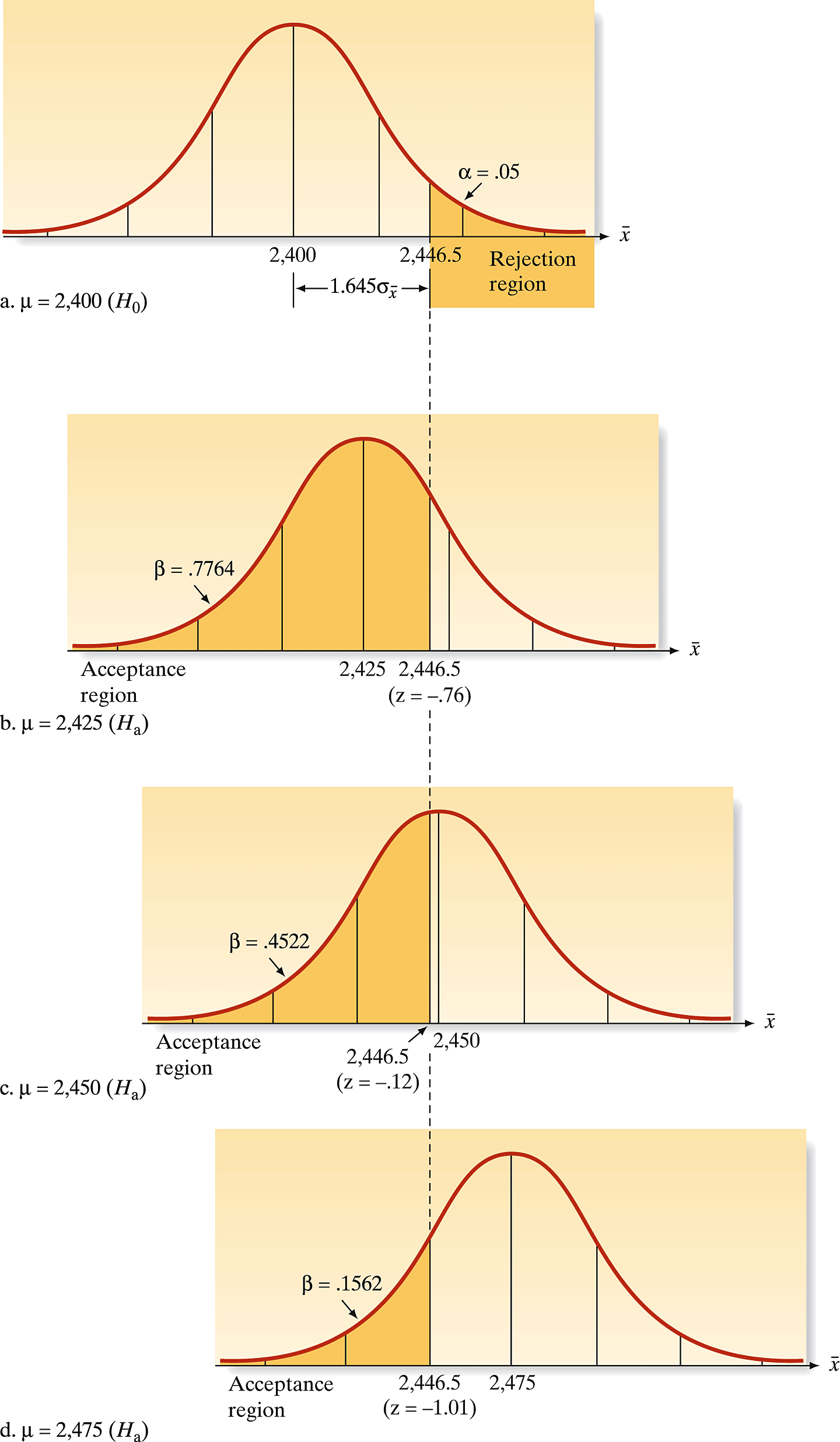
Manufacturing Scenario: Testing if new production process increases product strength
Null Hypothesis (\(H_0\)): No improvement in strength (\(\mu = 2400\))
Alternative Hypothesis (\(H_a\)): Process increases strength (\(\mu > 2400\))
Test Statistic: \[ z = \frac{\bar{x} - 2400}{\sigma / \sqrt{n}} \]
Standard Error: \(\sigma_{\bar{x}} = 28.267\) (based on historical data)
Rejection Region: For \(\alpha = 0.05\), reject \(H_0\) if \(z > 1.645\)
What We’re Testing: Is the observed improvement real, or just random variation?
Visualizing Error Probabilities
Understanding the Trade-off:
- Red Area (\(\alpha\)): The 5% chance of a false alarm - rejecting \(H_0\) when it’s actually true
- Type II Error (\(\beta\)): The risk of missing a real effect when \(H_a\) is true
- Power (\(1-\beta\)): Our ability to detect real improvements
Key Insight: As the true mean moves farther from \(2400\), our power increases and \(\beta\) decreases - we’re more likely to detect real improvements!
Calculating Type II Error Risk
When \(H_0\) is False: What’s our risk of missing the real effect?
- Type II Error (\(\beta\)): Probability of not rejecting \(H_0\) when it’s actually false
- Depends on: How far the true mean is from the null value
Example Calculation: If the true mean is 2425 (slight improvement)
\[ \beta = \operatorname{Prob}\left[\bar{x} < 2446.5 \mid \mu = 2425\right] = 0.7764 \]
Interpretation: We have a 77.6% chance of missing this small improvement! This shows why small effects are hard to detect.
Statistical Power: Getting It Right!
Power = 1 - \(\beta\): Our ability to detect real effects when they exist
- High Power: Good at finding real improvements
- Low Power: Often misses real effects
Why Power Matters:
- Medical Research: Need high power to detect treatment benefits
- Quality Control: Need balanced power to avoid false alarms
- Scientific Studies: Underpowered studies waste resources
Key Insight: Power increases as effects get larger and samples get bigger!
Worked Example 1: Medical Testing Error Analysis
Context: Medical diagnostic test with known error rates
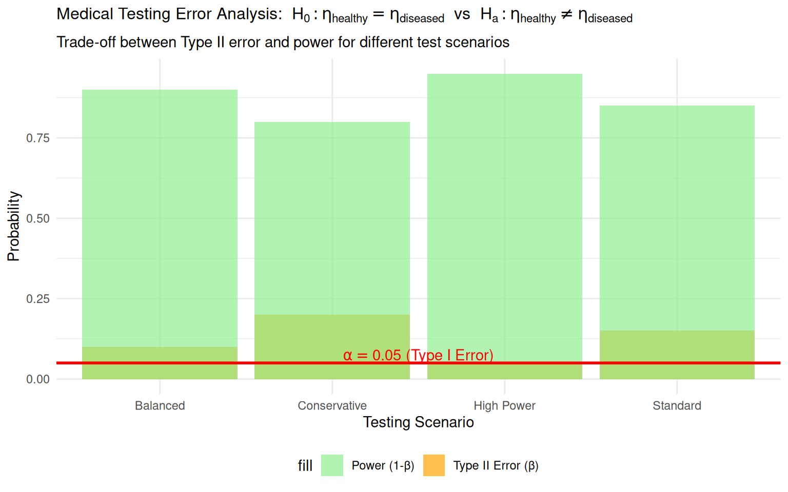
Worked Example 1: Formal Hypothesis Test Setup
- \(H_0\): Patient is healthy (no disease present)
- \(H_a\): Patient has disease (medical condition present)
- Type I Error (\(\alpha\)): False positive (healthy patient diagnosed as diseased)
- Type II Error (\(\beta\)): False negative (diseased patient diagnosed as healthy)
- Power (\(1-\beta\)): Correctly detecting disease when present
Error Probability Calculations:
- Scenario 1 (Conservative): \(\alpha = 0.05\), \(\beta = 0.20\), Power = 0.80
- Scenario 2 (Standard): \(\alpha = 0.05\), \(\beta = 0.15\), Power = 0.85
- Scenario 3 (Balanced): \(\alpha = 0.05\), \(\beta = 0.10\), Power = 0.90
- Scenario 4 (High Power): \(\alpha = 0.05\), \(\beta = 0.05\), Power = 0.95
Interpretation:
- Lower \(\beta\) values increase power but may require more sensitive tests
- Medical context often prioritizes minimizing \(\beta\) (false negatives)
- Trade-off between sensitivity and specificity
Worked Example 2: Quality Control Error Analysis
Context: Manufacturing process monitoring for defect rates
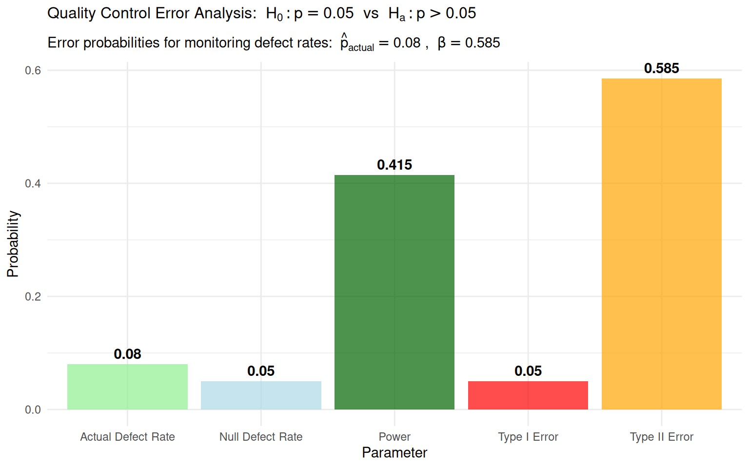
Worked Example 2: Formal Hypothesis Test Setup
- \(H_0\): \(p = 0.05\) (process operating at acceptable defect rate)
- \(H_a\): \(p > 0.05\) (process producing excessive defects)
- Sample: n=100 items monitored
- Rejection Region: \(\hat{p} > 0.05 + 1.645\sqrt{0.05(0.95)/100}\)
Error Probability Calculations:
Type I Error (\(\alpha\)): Probability of rejecting \(H_0\) when process is acceptable \[\alpha = 0.05\]
Type II Error (\(\beta\)): Probability of accepting \(H_0\) when actual defect rate is 8% \[\beta = P(\hat{p} < 0.0858 \mid p = 0.08) = 0.585\]
Power (\(1-\beta\)): Probability of detecting process deterioration \[\text{Power} = 1 - 0.585 = 0.415\]
Practical Implications:
- Current test has only 41.5% chance of detecting 8% defect rate
- May need larger sample size or lower \(\alpha\) for better detection
- Quality control requires balancing error rates with monitoring costs
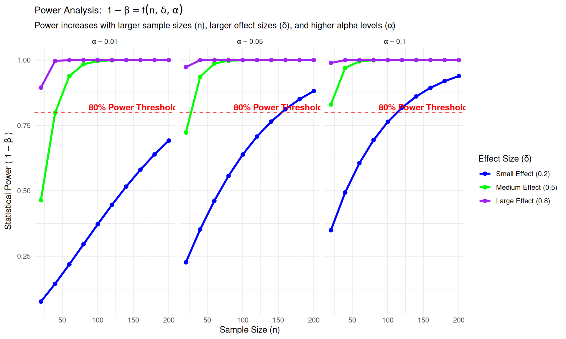
What Determines Statistical Power?
Effect Size (\(\delta\)): How big is the real difference? \[\delta = |\mu_a - \mu_0|\]
- Large effects: Easy to detect (high power)
- Small effects: Hard to detect (low power)
Sample Size (\(n\)): How many observations do we have?
- Large samples: More precise estimates (high power)
- Small samples: More uncertainty (low power)
Significance Level (\(\alpha\)): How strict are we about false alarms?
- Conservative (\(\alpha=0.01\)): Fewer false alarms, lower power
- Liberal (\(\alpha=0.10\)): More false alarms, higher power
Population Variability (\(\sigma\)): How noisy is our data?
- Low variability: Clear signal (high power)
- High variability: Hard to see signal (low power)
Power Analysis Visualization
Practical Power Analysis: Planning Better Studies
# How much power do I have with n=30?
power.t.test(n = 30, delta = 0.5, sd = 1, sig.level = 0.05, type = "one.sample")
     One-sample t test power calculation

              n = 30
          delta = 0.5
             sd = 1
      sig.level = 0.05
          power = 0.7539627
    alternative = two.sided
# How many subjects do I need for 80% power?
power.t.test(power = 0.80, delta = 0.5, sd = 1, sig.level = 0.05, type = "one.sample")
     One-sample t test power calculation

              n = 33.3672
          delta = 0.5
             sd = 1
      sig.level = 0.05
          power = 0.8
    alternative = two.sided
Real-World Interpretation:
“Our study with 30 participants has 80% power to detect a medium effect. This means if the treatment really works, we have an 80% chance of finding it.”