flowchart LR
    %% Styling definitions
    classDef start fill:#FFFACD,stroke:#FF8C00,stroke-width:2px,color:#000
    classDef decision fill:#E6F3FF,stroke:#1E88E5,stroke-width:2px,color:#000
    classDef action fill:#E8F5E9,stroke:#43A047,stroke-width:2px,color:#000
    classDef endStyle fill:#FFEBEE,stroke:#E53935,stroke-width:2px,color:#000

    %% Nodes
    A([Start]):::start
    B{State H₀: Specified Distribution}:::decision
    C{Calculate Expected Counts}:::decision
    D{Compute χ² Statistic}:::decision
    E{Compare to χ² Distribution}:::decision
    F[Reject H₀<br/>Poor fit to distribution]:::action
    G[Fail to reject H₀<br/>Good fit to distribution]:::action
    H[Interpret Practical Significance]:::endStyle

    %% Flow connections
    A --> B
    B --> C
    C --> D
    D --> E
    E -->|p < α| F
    E -->|p ≥ α| G
    F --> H
    G --> H
Day 33
Math 216: Statistical Thinking
Bastola
Chi-Square Goodness of Fit Test
Key Question: How do we test if categorical data fits a specific distribution? Welcome to the chi-square goodness of fit test!
- When to Use: Testing if observed categorical counts match expected proportions
- Real-World Applications:
- Testing fairness of dice, coins, or games
- Checking if survey responses match population demographics
- Verifying if genetic ratios follow Mendelian inheritance
Core Concept: Compare observed frequencies with expected frequencies under \(H_0\)
The Chi-Square Test Statistic
How We Measure Fit:
\[\chi^2 = \sum_{j=1}^{k} \frac{(O_j - E_j)^2}{E_j}\]
Where:
- \(O_j\) = Observed count in category \(j\)
- \(E_j\) = Expected count in category \(j\) under \(H_0\)
- \(k\) = Number of categories
Intuition: Large \(\chi^2\) values indicate poor fit between observed and expected counts
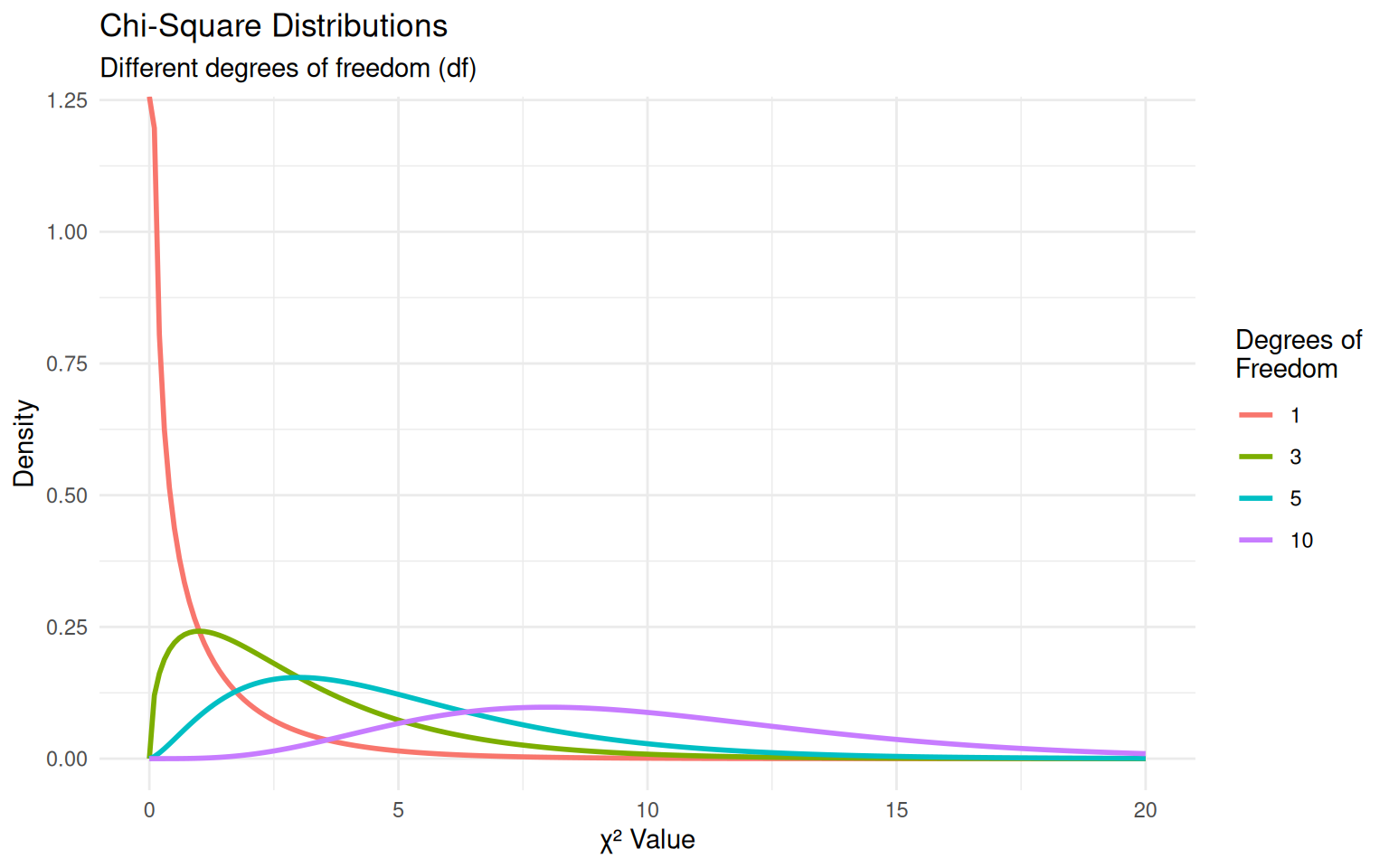
Distribution: Under \(H_0\), \(\chi^2\) follows a chi-square distribution with \(df = k - 1\)
Chi-Square Distribution Properties
Goodness of Fit Test Framework
Example 1: Testing a Fair Die
Research Question: Is this six-sided die fair?
Data: 60 rolls with observed counts:
| Outcome | 1 | 2 | 3 | 4 | 5 | 6 |
|---|---|---|---|---|---|---|
| Observed | 12 | 7 | 14 | 15 | 4 | 8 |
Hypotheses:
- \(H_0\): Die is fair (all outcomes equally likely)
- \(H_a\): Die is not fair (outcomes not equally likely)
Expected: Each side = \(60 \times \frac{1}{6} = 10\)
Die Fairness Test: R Implementation
# Observed die roll frequencies
observed_die <- c(12, 7, 14, 15, 4, 8)

# Expected probabilities for fair die
expected_probs <- rep(1/6, 6)

# Perform chi-square test
die_test <- chisq.test(x = observed_die, p = expected_probs)
die_test
    Chi-squared test for given probabilities

data:  observed_die
X-squared = 9.4, df = 5, p-value = 0.09413
Detailed Results:Chi-square statistic = 9.4 Degrees of freedom = 5 P-value = 0.0941 Decision: FAIL TO REJECT H₀ (p ≥ 0.05)
Conclusion: No evidence the die is unfairVisualizing Die Fairness Test

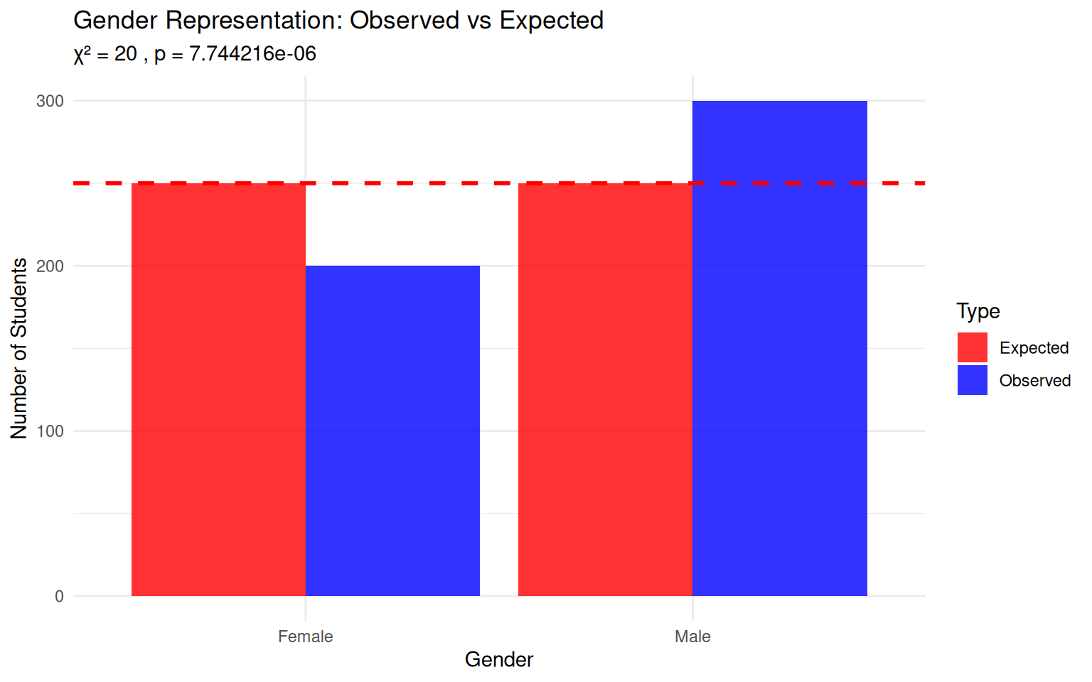
Example 2: Gender Representation in STEM
Research Question: Does a university STEM program have equal gender representation?
Background: Regional expectation is 50:50 male-to-female ratio
Data: 500 students enrolled
- Female: 200 students
- Male: 300 students
Hypotheses:
- \(H_0\): \(p_f = p_m = \frac{1}{2}\) (equal representation)
- \(H_a\): \(p_f \neq p_m\) (unequal representation)
Expected: Each gender = \(500 \times \frac{1}{2} = 250\)
Gender Representation Test: R Implementation
# Gender representation data
observed_gender <- c(200, 300)  # Female, Male
expected_probs_gender <- c(0.5, 0.5)

# Perform chi-square test
gender_test <- chisq.test(x = observed_gender, p = expected_probs_gender)
gender_test
    Chi-squared test for given probabilities

data:  observed_gender
X-squared = 20, df = 1, p-value = 7.744e-06
Detailed Results:Chi-square statistic = 20 Degrees of freedom = 1 P-value = 8e-06 Decision: REJECT H₀ (p < 0.05)
Conclusion: Evidence of unequal gender representationVisualizing Gender Representation
Chi-Square Test Assumptions
Critical Requirements for Valid Testing:
- Independence: Observations must be independent of each other
- Sample Size: All expected counts should be ≥ 5
- Categorical Data: Variables must be categorical (not continuous)
- Fixed Total: The total sample size is fixed
When Assumptions Fail:
- Small expected counts → Use Fisher’s exact test
- Dependent observations → Different statistical methods needed
- Continuous data → Use different tests (t-tests, ANOVA, etc.)
Rule of Thumb: If any \(E_j < 5\), consider combining categories
Goodness of Fit Test Summary
- State Hypotheses: Clearly define \(H_0\) and \(H_a\)
- Calculate Expected: \(E_j = n \times p_j\) under \(H_0\)
- Compute Test Statistic: \(\chi^2 = \sum \frac{(O_j - E_j)^2}{E_j}\)
- Determine Degrees of Freedom: \(df = k - 1\)
- Find P-value: Compare \(\chi^2\) to chi-square distribution
- Make Decision: Reject \(H_0\) if p-value < α
- Interpret Results: Practical significance and limitations
Key Insight: Chi-square tests tell us if patterns are systematic or just random variation!
R Toolkit: Chi-Square Goodness of Fit
Basic Chi-Square Test
# Test if observed counts match expected proportions
chisq.test(x = observed_counts, p = expected_proportions)
Example Applications
# Testing fair coin (50:50)
coin_test <- chisq.test(c(45, 55), p = c(0.5, 0.5))

# Testing genetic ratios (3:1)
genetic_test <- chisq.test(c(75, 25), p = c(0.75, 0.25))

# Testing uniform distribution
uniform_test <- chisq.test(c(12, 15, 18, 10),
                          p = c(0.25, 0.25, 0.25, 0.25))