flowchart LR
    %% Styling definitions
    classDef start fill:#FFFACD,stroke:#FF8C00,stroke-width:2px,color:#000
    classDef decision fill:#E6F3FF,stroke:#1E88E5,stroke-width:2px,color:#000
    classDef action fill:#E8F5E9,stroke:#43A047,stroke-width:2px,color:#000
    classDef endStyle fill:#FFEBEE,stroke:#E53935,stroke-width:2px,color:#000

    %% Nodes
    %% Text wrapped to be tall/narrow to save horizontal space
    A(["Start:<br/>Contingency<br/>Table"]):::start
    B{"State H₀:<br/>Variables<br/>Indep."}:::decision
    C{"Calculate<br/>Expected<br/>Counts"}:::decision
    D{"Compute<br/>χ² Statistic"}:::decision
    E{"Compare to<br/>χ² Dist."}:::decision
    F["Reject H₀<br/>Evidence of<br/>Relationship"]:::action
    G["Fail to<br/>Reject H₀<br/>No Evidence"]:::action
    H["Interpret<br/>Association"]:::endStyle

    %% Flow connections
    A --> B
    B --> C
    C --> D
    D --> E
    E -->|p < α| F
    E -->|p ≥ α| G
    F --> H
    G --> H
Day 34
Math 216: Statistical Thinking
Bastola
Chi-Square Test of Independence
Key Question: Are two categorical variables related, or are they independent?
When to Use: Testing association between two categorical variables
Real-World Applications:
- Does vaccination status affect flu contraction?
- Is political affiliation related to policy preferences?
- Are smoking habits associated with lung disease?
Core Concept: Compare observed joint frequencies with expected frequencies under independence
Contingency Tables: The Foundation
Understanding Two-Way Tables:
| Column 1 | Column 2 | … | Column c | Total | |
|---|---|---|---|---|---|
| Row 1 | \(n_{11}\) | \(n_{12}\) | … | \(n_{1c}\) | \(r_1\) |
| Row 2 | \(n_{21}\) | \(n_{22}\) | … | \(n_{2c}\) | \(r_2\) |
| … | \(\vdots\) | \(\vdots\) | … | \(\vdots\) | \(\vdots\) |
| Row r | \(n_{r1}\) | \(n_{r2}\) | … | \(n_{rc}\) | \(r_r\) |
| Total | \(c_1\) | \(c_2\) | … | \(c_c\) | \(n\) |
Where:
- \(n_{ij}\) = Observed count in cell (i,j)
- \(r_i\) = Row total for row i
- \(c_j\) = Column total for column j
- \(n\) = Grand total
Key Insight: If variables are independent, cell frequencies should follow row × column proportions
Test of Independence Framework
The Chi-Square Test Statistic
How We Measure Association:
\[\chi^2 = \sum_{i=1}^{r} \sum_{j=1}^{c} \frac{(O_{ij} - E_{ij})^2}{E_{ij}}\]
Where:
- \(O_{ij}\) = Observed count in cell (i,j)
- \(E_{ij}\) = Expected count under independence
- \(E_{ij} = \frac{r_i \times c_j}{n}\)
Degrees of Freedom: \[ df = (r - 1) \times (c - 1) \]
Intuition: Large \(\chi^2\) values indicate strong association between variables
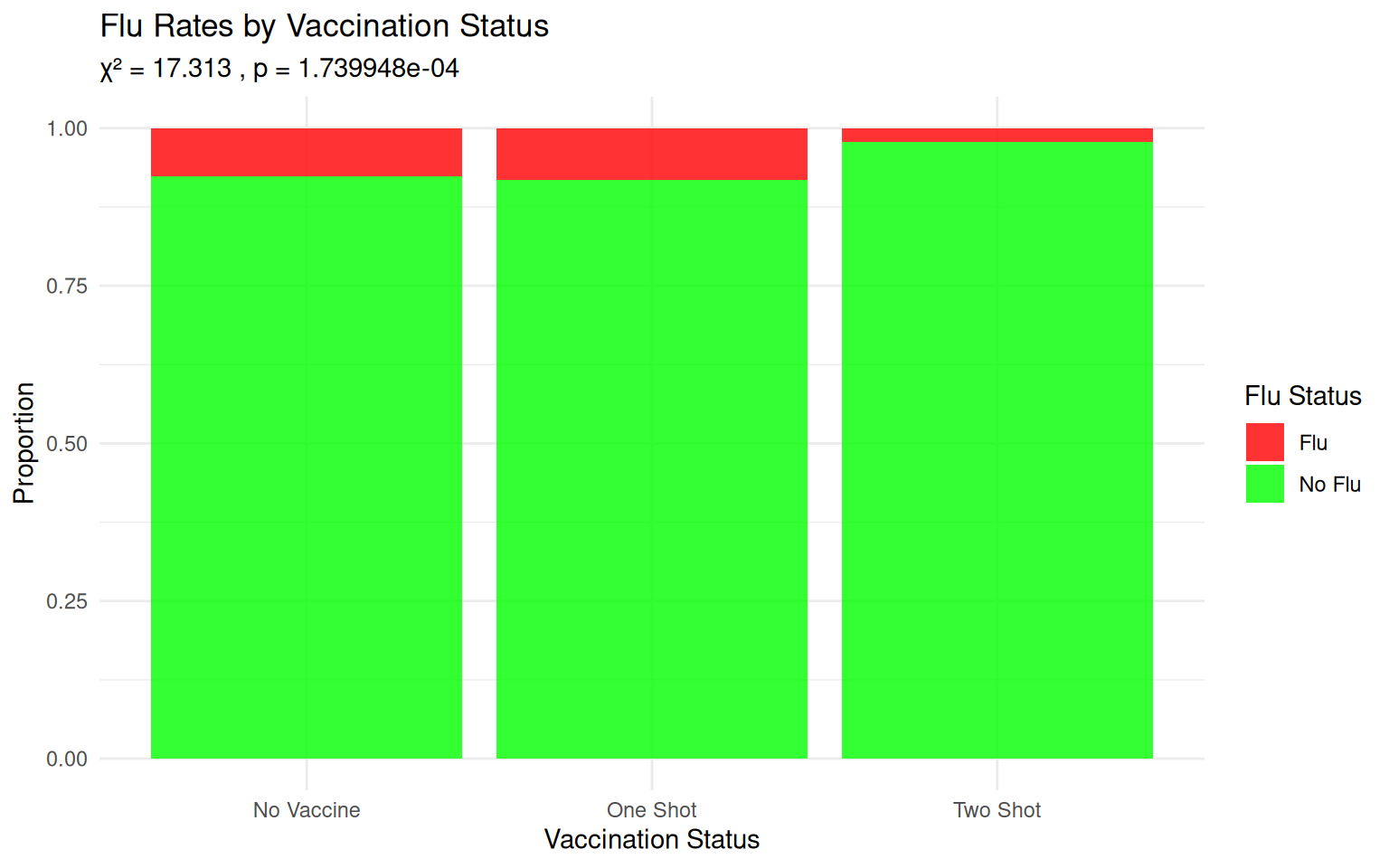
Example 1: Flu Vaccine Effectiveness
Research Question: Does flu vaccination reduce flu contraction?
Data: 1000 individuals surveyed
| Status | No Vaccine | One Shot | Two Shot | Total |
|---|---|---|---|---|
| Flu | 24 | 9 | 13 | 46 |
| No Flu | 289 | 100 | 565 | 954 |
| Total | 313 | 109 | 578 | 1000 |
Hypotheses:
- \(H_0\): Flu status and vaccination status are independent
- \(H_a\): Flu status and vaccination status are dependent
Expected: If independent, flu rates should be similar across vaccination groups
Vaccine Effectiveness Test: R Implementation
# Create contingency table for vaccine data
flu_vaccine_data <- matrix(c(24, 9, 13, 289, 100, 565),
                          nrow = 2, byrow = TRUE,
                          dimnames = list(c("Flu", "No Flu"),
                                         c("No Vaccine", "One Shot", "Two Shot")))

# Perform chi-square test
vaccine_test <- chisq.test(flu_vaccine_data, correct = FALSE)
vaccine_test
    Pearson's Chi-squared test

data:  flu_vaccine_data
X-squared = 17.313, df = 2, p-value = 0.000174
Detailed Results:Chi-square statistic = 17.313 Degrees of freedom = 2 P-value = 1.739948e-04 Expected counts under independence: No Vaccine One Shot Two Shot
Flu 14.4 5.01 26.59
No Flu 298.6 103.99 551.41
Decision: REJECT H₀ (p < 0.05)
Conclusion: Evidence that vaccination affects flu contraction
Visualizing Vaccine Effectiveness
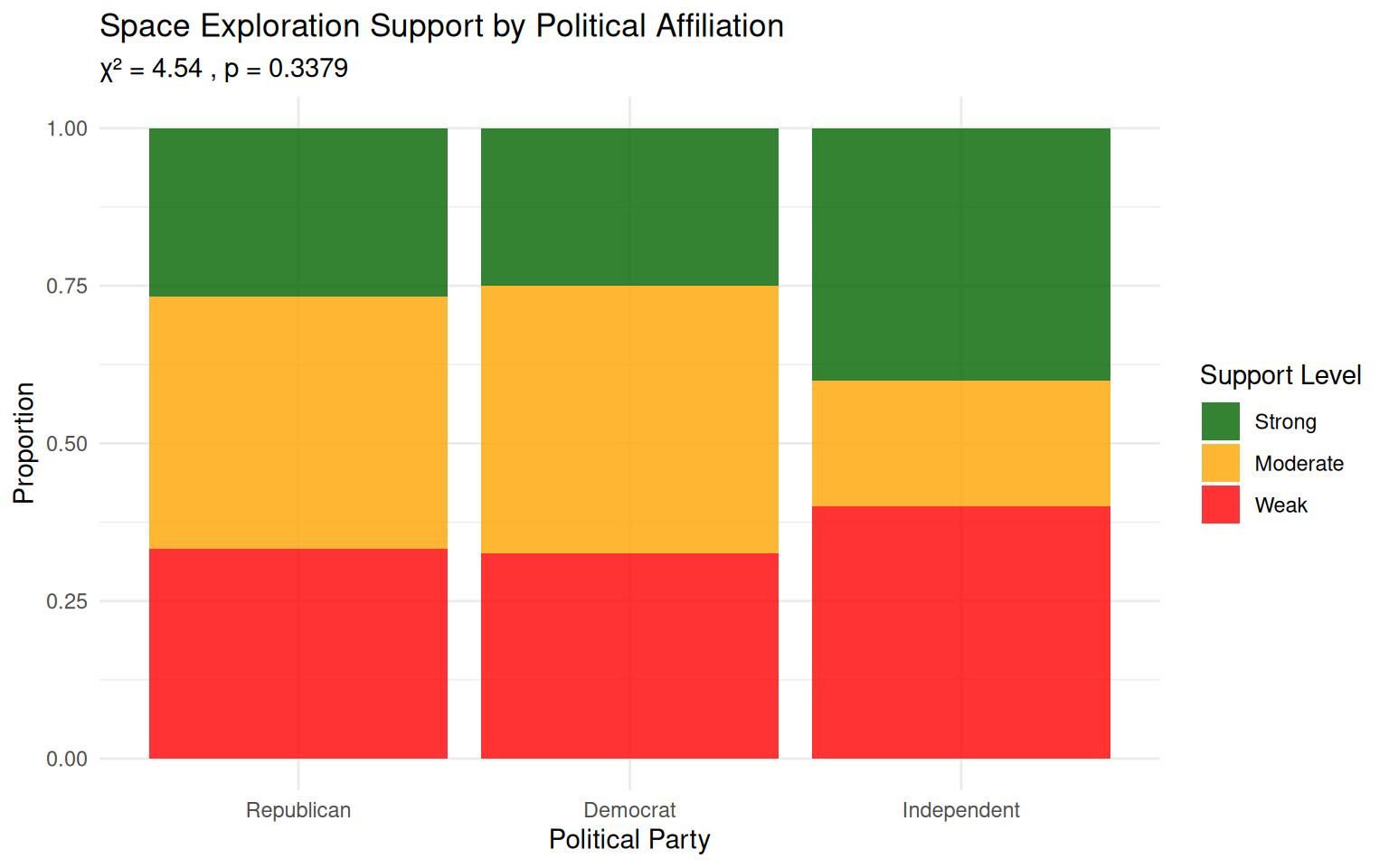
Example 2: Political Views & Space Exploration
Research Question: Is political affiliation related to support for space exploration?
Data: 100 individuals surveyed
| Support Level | Republican | Democrat | Independent | Total |
|---|---|---|---|---|
| Strong | 8 | 10 | 12 | 30 |
| Moderate | 12 | 17 | 6 | 35 |
| Weak | 10 | 13 | 12 | 35 |
| Total | 30 | 40 | 30 | 100 |
Hypotheses:
- \(H_0\): Political affiliation and space support are independent
- \(H_a\): Political affiliation and space support are dependent
Expected: If independent, support patterns should be similar across political groups
Political Views Test: R Implementation
# Create contingency table for political views
politics_data <- matrix(c(8, 10, 12, 12, 17, 6, 10, 13, 12),
                       nrow = 3, byrow = TRUE,
                       dimnames = list(c("Strong", "Moderate", "Weak"),
                                      c("Republican", "Democrat", "Independent")))

# Perform chi-square test
politics_test <- chisq.test(politics_data, correct = FALSE)
politics_test
    Pearson's Chi-squared test

data:  politics_data
X-squared = 4.5397, df = 4, p-value = 0.3379
Detailed Results:Chi-square statistic = 4.54 Degrees of freedom = 4 P-value = 0.3379 Expected counts under independence: Republican Democrat Independent
Strong 9.0 12 9.0
Moderate 10.5 14 10.5
Weak 10.5 14 10.5
Decision: FAIL TO REJECT H₀ (p ≥ 0.05)
Conclusion: No evidence of relationship between politics and space support
Visualizing Political Views Data
Test of Independence Assumptions
Critical Requirements for Valid Testing:
- Independence: Observations must be independent of each other
- Sample Size: All expected counts should be ≥ 5
- Categorical Data: Both variables must be categorical
- Random Sampling: Data should come from random sampling
When Assumptions Fail:
- Small expected counts → Use Fisher’s exact test
- Continuous variables → Use correlation or regression
Rule of Thumb: If >20% of cells have \(E_{ij} < 5\), consider combining categories
Test of Independence Summary
Your Testing Checklist:
- State Hypotheses: \(H_0\): independence vs \(H_a\): dependence
- Calculate Expected: \(E_{ij} = \frac{r_i \times c_j}{n}\)
- Compute Test Statistic: \(\chi^2 = \sum \frac{(O_{ij} - E_{ij})^2}{E_{ij}}\)
- Determine Degrees of Freedom: \(df = (r-1)(c-1)\)
- Find P-value: Compare \(\chi^2\) to chi-square distribution
- Make Decision: Reject \(H_0\) if p-value < α
- Interpret Results: Practical significance and effect size
Key Insight: Chi-square tests reveal whether patterns in contingency tables reflect real relationships!
R Toolkit: Chi-Square Test of Independence
Goodness of Fit vs Test of Independence
Key Differences:
| Aspect | Goodness of Fit | Test of Independence |
|---|---|---|
| Purpose | Test if data fits specified distribution | Test if two variables are related |
| Variables | One categorical variable | Two categorical variables |
| Expected | Based on specified probabilities | Based on row × column proportions |
| df Formula | \(k - 1\) | \((r-1)(c-1)\) |
| H₀ | Data follows specified distribution | Variables are independent |
Common Ground:
- Both use chi-square test statistic
- Both require categorical data out.wi