Day 36

Math 216: Statistical Thinking

Bastola

Simple Linear Regression: Model Estimation

Key Question: How do we actually estimate the “best” regression line from our data?

  • Recap: We learned to estimate the simple linear regression line \(\hat{y} = \hat{\beta}_0 + \hat{\beta}_1 x\) from a sample
  • Deeper Analysis: To go beyond basic fitting, we need to understand key regression assumptions
  • Real-World Goal: Build models that not only fit data but also provide reliable predictions

Building on Our Journey: From correlation to prediction - we’re moving from describing relationships to building predictive models!

The Five-Step Regression Framework

Key Question: What’s the systematic process for building and validating regression models?

  • Step 1: Hypothesize the deterministic component that relates mean \(E(y)\) to independent variable \(x\)
  • Step 2: Use sample data to estimate unknown parameters in the model
  • Step 3: Specify the probability distribution of random error and estimate its standard deviation
  • Step 4: Statistically evaluate the usefulness of the model
  • Step 5: Use the validated model for prediction, estimation, and decision-making

Real-World Insight: This systematic approach ensures our models are both statistically sound and practically useful!

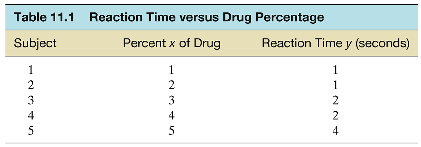
Real-World Example: Drug Reaction Time Study

Research Question: How does drug concentration affect reaction time?

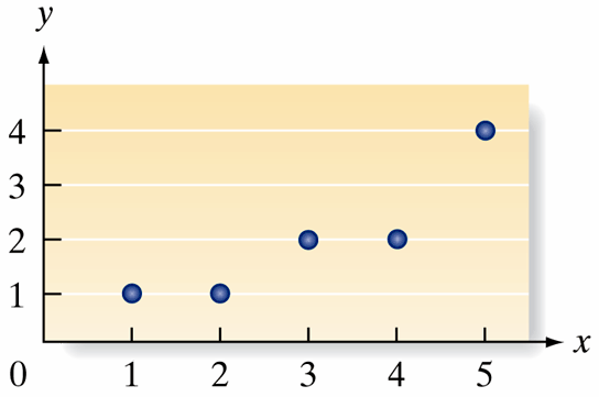
  • Scenario: Medical researchers want to predict reaction time \(y\) based on drug percentage \(x\) in bloodstream
  • Data: Collected from five subjects (simplified for learning)
  • Goal: Build a model to understand and predict drug effects

Key Insight: Even simple experiments can reveal important relationships - and help us understand the regression process step by step!

Step 1: Hypothesize the Deterministic Component

Key Question: What mathematical relationship do we expect between drug percentage and reaction time?

  • Focus: Straight-line models (linear relationships)
  • Relationship: Mean response time to drug percentage

Our Hypothesis: We assume the model relating mean response time \(E(y)\) to drug percentage \(x\):

\[ H: E(y) = \beta_0 + \beta x \longleftarrow \begin{aligned} & \text{The true unknown relationship} \\ & \text{between } x \text{ and } Y \text{ is a straight line} \end{aligned} \]

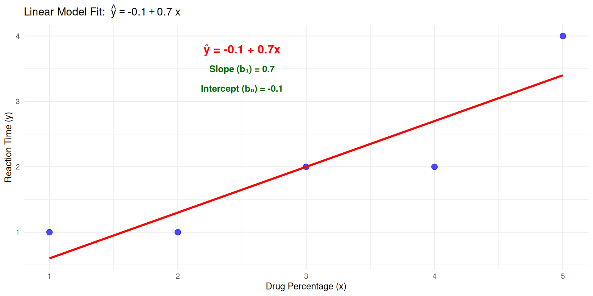
Step 2: Estimate Model Parameters from Sample Data

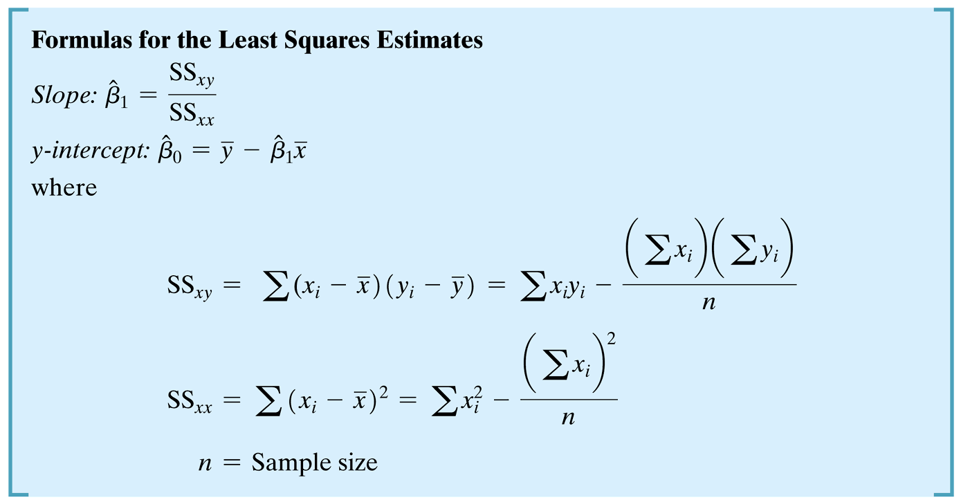
Key Question: How do we find the “best” values for \(\beta_0\) and \(\beta_1\) using our sample data?

  • Challenge: Use our five observations to estimate the unknown \(y\)-intercept \(\beta_0\) and slope \(\beta_1\)
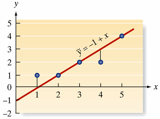
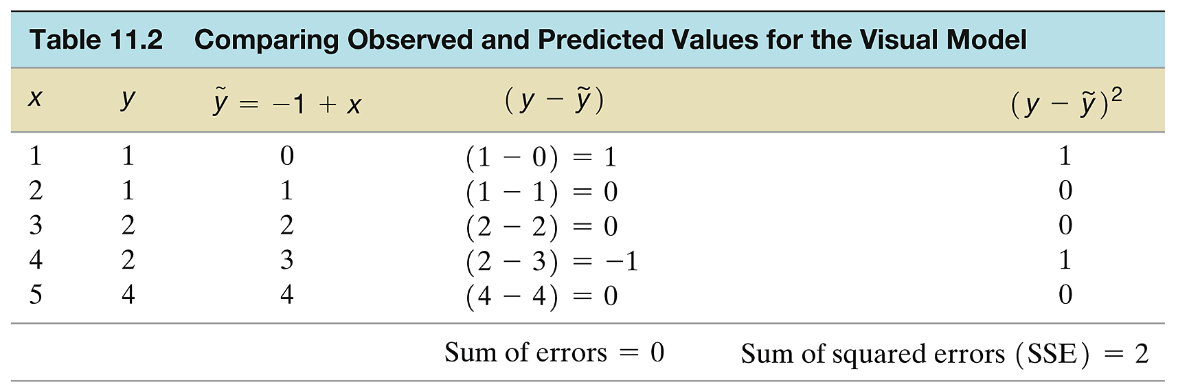
  • Method: Least squares estimation - finding the line that minimizes prediction errors
  • Goal: Transform our hypothesis into concrete parameter estimates

Five-Step Regression Framework

%%{init: {"theme": "base", "themeVariables": {"fontSize": "24px", "fontFamily": "Arial", "lineColor": "#333"}}}%%

flowchart LR
    %% --- Styling Definitions ---
    classDef start fill:#FFFACD,stroke:#FF8C00,stroke-width:2px,color:#000
    classDef step fill:#E6F3FF,stroke:#1E88E5,stroke-width:2px,color:#000
    classDef action fill:#E8F5E9,stroke:#43A047,stroke-width:2px,color:#000
    classDef endStyle fill:#FFEBEE,stroke:#E53935,stroke-width:2px,color:#000

    %% --- Five-Step Process ---
    A([Start: Research Question]):::start
    B["Step 1: Hypothesize<br/>E(y) = β₀ + β₁x"]:::step
    C["Step 2: Estimate<br/>Find b₀, b₁ via Least Squares"]:::step
    D["Step 3: Specify Distribution<br/>ε ~ N(0, σ²)"]:::step
    E["Step 4: Evaluate Model<br/>Test H₀: β₁ = 0"]:::step
    F["Step 5: Use Model<br/>Prediction & Estimation"]:::step
    G["Validated Model<br/>Ready for Application"]:::endStyle

    %% --- Connections ---
    A --> B
    B --> C
    C --> D
    D --> E
    E --> F
    F --> G

    %% --- Visual Polish ---
    linkStyle default stroke:#333,stroke-width:2px;

Deriving Slope and Intercept from Correlation

Key Question: How can we derive the regression coefficients directly from the correlation coefficient?

  • Relationship between correlation and regression: \[ b_1 = r \cdot \frac{s_y}{s_x} \] \[ b_0 = \bar{y} - b_1\bar{x} \]

Verification with our drug reaction data

# Define the data (same as earlier)
x <- c(1, 2, 3, 4, 5)
y <- c(1, 1, 2, 2, 4)

# Fit linear model for comparison
mod <- lm(y ~ x)

# Calculate correlation and standard deviations
drug_corr <- cor(x, y)
sd_x <- sd(x)
sd_y <- sd(y)
mean_x <- mean(x)
mean_y <- mean(y)

# Derive slope and intercept from correlation
b1_from_r <- drug_corr * (sd_y / sd_x)
b0_from_r <- mean_y - b1_from_r * mean_x

# Compare with lm() results
round(drug_corr, 4) # correlation
[1] 0.9037
round(b1_from_r, 4) # slope
[1] 0.7
round(b0_from_r, 4) # y-intercept
[1] -0.1
coef(mod) # LM results
(Intercept)           x 
       -0.1         0.7 

Implementing Regression in R


Call:
lm(formula = y ~ x, data = data)

Residuals:
         1          2          3          4          5 
 4.000e-01 -3.000e-01 -5.551e-17 -7.000e-01  6.000e-01 

Coefficients:
            Estimate Std. Error t value Pr(>|t|)  
(Intercept)  -0.1000     0.6351  -0.157   0.8849  
x             0.7000     0.1915   3.656   0.0354 *
---
Signif. codes:  0 '***' 0.001 '**' 0.01 '*' 0.05 '.' 0.1 ' ' 1

Residual standard error: 0.6055 on 3 degrees of freedom
Multiple R-squared:  0.8167,    Adjusted R-squared:  0.7556 
F-statistic: 13.36 on 1 and 3 DF,  p-value: 0.03535

library(ggplot2)
ggplot(data, aes(x = x, y = y)) +
  geom_point() +  # Add points
  geom_smooth(method = "lm", se = FALSE) +  
  ggtitle("Linear Model Fit") +
  theme_minimal()