Day 37

Math 216: Statistical Thinking

Bastola

Key Assumptions for Linear Regression

Key Question: What conditions must be met for our regression results to be valid?

• Simple Linear Regression Model:

  • \(y = \beta_0 + \beta_1 x + \varepsilon\)

• Four Critical Assumptions:

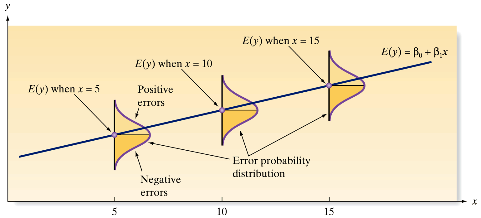
  1. Mean of Errors (\(\varepsilon\)): The mean of the probability distribution of \(\varepsilon\) is 0, aligning the expected value of \(y\) with \(\beta_0 + \beta_1 x\) for any \(x\)
  2. Constant Variance: The variance of \(\varepsilon\) is constant across all values of \(x\), denoted as \(\sigma^2\)
  3. Normal Distribution of Errors: \(\varepsilon\) follows a normal distribution
  4. Independence of Errors: The errors associated with different \(y\) values are independent

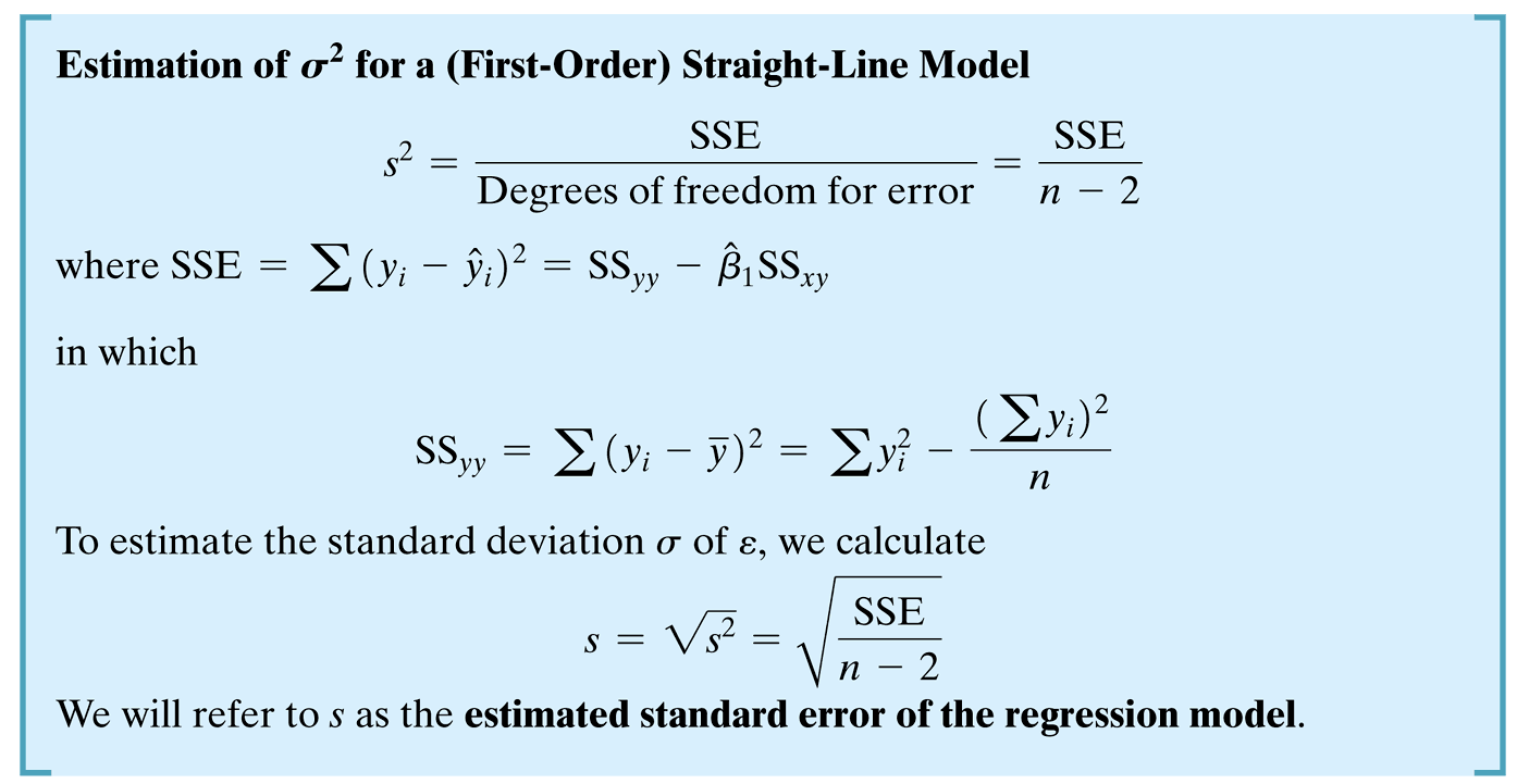
Constant Variance

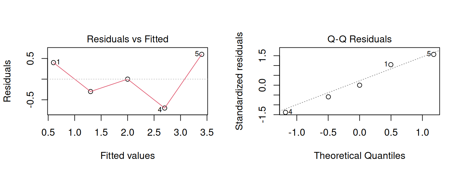
How do we check regression assumptions?

# Fit model and check assumptions
par(mfrow = c(1, 2))
plot(mod, which = 1:2)

Interpreting Diagnostic Plots:

• Residuals vs Fitted: Check constant variance (no patterns)
• Normal Q-Q: Check normality (points follow straight line)

Call:
lm(formula = y ~ x)

Residuals:
         1          2          3          4          5 
 4.000e-01 -3.000e-01 -5.551e-17 -7.000e-01  6.000e-01 

Coefficients:
            Estimate Std. Error t value Pr(>|t|)  
(Intercept)  -0.1000     0.6351  -0.157   0.8849  
x             0.7000     0.1915   3.656   0.0354 *
---
Signif. codes:  0 '***' 0.001 '**' 0.01 '*' 0.05 '.' 0.1 ' ' 1

Residual standard error: 0.6055 on 3 degrees of freedom
Multiple R-squared:  0.8167,    Adjusted R-squared:  0.7556 
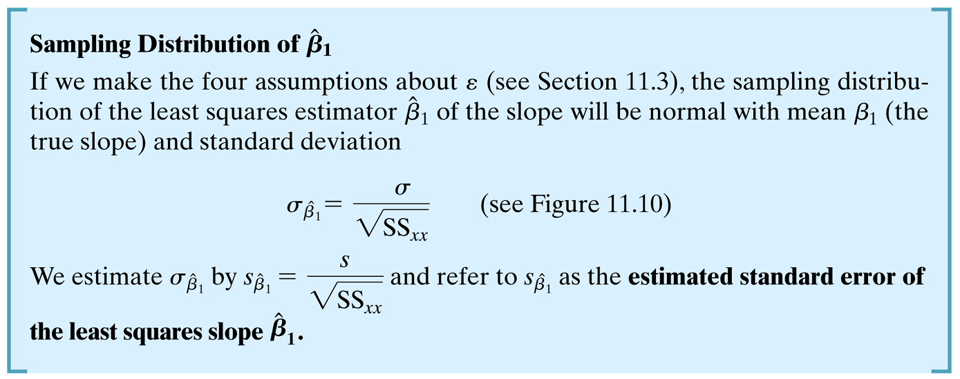
F-statistic: 13.36 on 1 and 3 DF,  p-value: 0.03535

Making Inferences About the Slope \(\beta_1\)

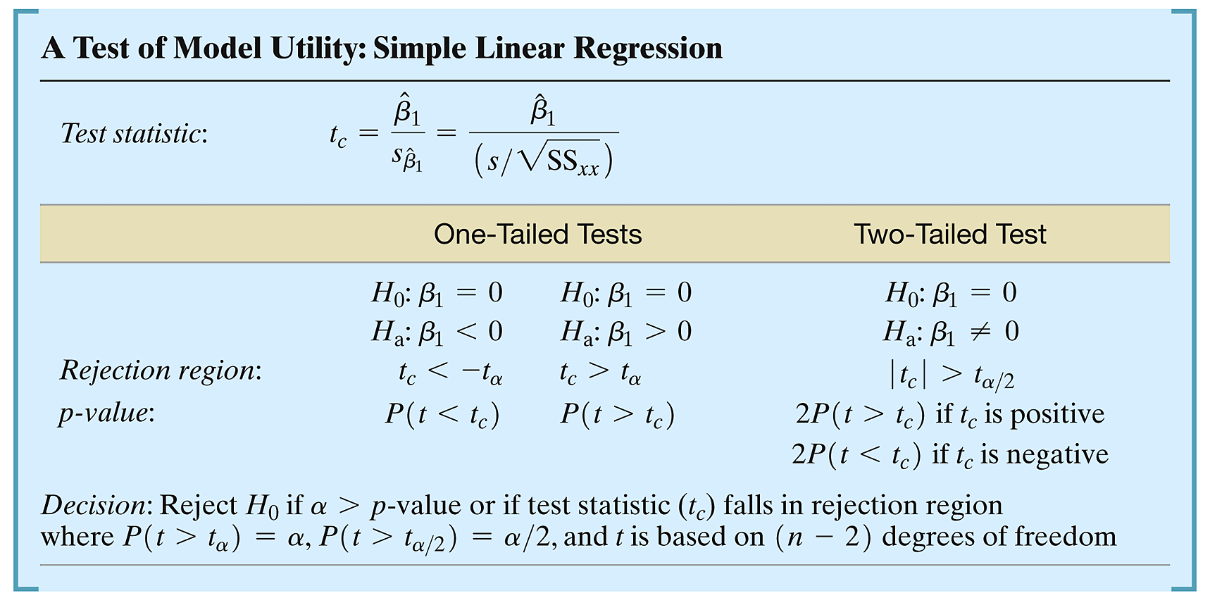
Key Question: Is the relationship we found statistically significant, or just random chance?

• Objective: Assess the significance of the slope \(\beta_1\) to understand if \(x\) truly helps predict \(y\)
• Statistical Test:
  • Null Hypothesis (\(H_0\)): \(\beta_1 = 0\) (No relationship - changes in \(x\) don’t affect \(y\))
  • Alternative Hypothesis (\(H_a\)): \(\beta_1 \neq 0\) (Significant relationship - \(x\) does affect \(y\))
• Using R for Hypothesis Testing:
  • Perform t-tests to decide whether to reject \(H_0\)
  • A significant \(p\)-value (\(< \alpha\)) indicates a meaningful contribution of \(x\) to predicting \(y\)

Real-World Insight: This test tells us if our predictor variable is actually useful, or if we’re just seeing patterns in random noise!

Practical Steps Using R

Key Question: How do we actually test for slope significance in R?

• Conducting the Test:
  1. Estimate \(\hat{\beta}_0\) and \(\hat{\beta}_1\) using the least squares method
  2. Compute the standard error and perform a t-test to check the significance of \(\hat{\beta}_1\)
  3. Interpret the results: A significant test suggests that changes in \(x\) systematically relate to changes in \(y\)

Real-World Application: This process transforms our regression output into actionable insights about variable relationships!

Hypothesis Testing

How can we make a decision of this hypothesis test using R?

Estimate Std. Error t value Pr(>|t|) (Intercept) -0.1 0.6350853 -0.1574592 0.8848840 x 0.7 0.1914854 3.6556308 0.0353528

Regression Hypothesis Testing Framework

%%{init: {"theme": "base", "themeVariables": {"fontSize": "30px", "fontFamily": "Arial", "lineColor": "#333"}}}%%

flowchart LR
    %% --- Styling Definitions ---
    classDef start fill:#FFFACD,stroke:#FF8C00,stroke-width:2px,color:#000
    classDef decision fill:#E6F3FF,stroke:#1E88E5,stroke-width:2px,color:#000
    classDef action fill:#E8F5E9,stroke:#43A047,stroke-width:2px,color:#000
    classDef endStyle fill:#FFEBEE,stroke:#E53935,stroke-width:2px,color:#000

    %% --- Nodes ---
    %% Using <br/> to balance width and height
    A([Start:<br/>Regression Model]):::start
    B{"State Hypotheses<br/>H₀: β₁ = 0<br/>vs<br/>Hₐ: β₁ ≠ 0"}:::decision
    C{"Calculate Statistic<br/>t = b₁ / SE(b₁)"}:::decision
    D{"Compute p-value<br/>(t-dist)"}:::decision
    E{"Compare p-value<br/>to α = 0.05"}:::decision
    F["Reject H₀<br/>Significant"]:::action
    G["Fail to Reject H₀<br/>No Evidence"]:::action
    H["Interpret<br/>Results"]:::endStyle

    %% --- Connections ---
    A --> B
    B --> C
    C --> D
    D --> E
    E -->|p < .05| F
    E -->|p ≥ .05| G
    F --> H
    G --> H

    %% --- Visual Polish ---
    linkStyle default stroke:#333,stroke-width:2px;

Confidence Intervals

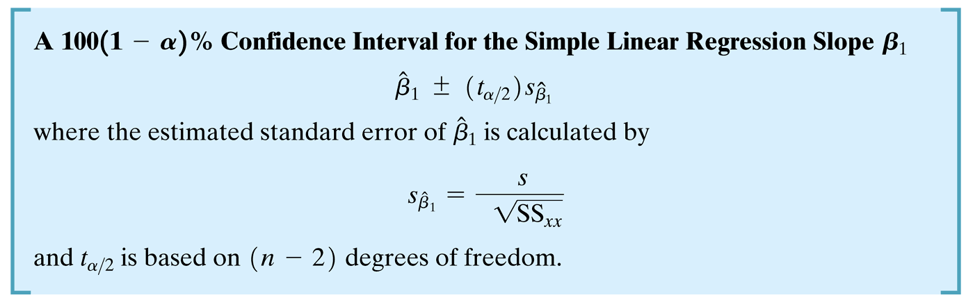
Confidence Intervals in R

                  2.5 %   97.5 %
(Intercept) -2.12112485 1.921125
x            0.09060793 1.309392