Day 40

Math 216: Statistical Thinking

Bastola

Blood Alcohol Content (BAC)

X	ID_OSU	Gender	Weight	Beers	BAC
1	1	female	132	5	0.100
2	2	female	128	2	0.030
3	3	female	110	9	0.190
4	4	male	192	8	0.120
5	5	male	172	3	0.040
6	6	female	250	7	0.095
7	7	female	125	3	0.070
8	8	male	175	5	0.060
9	9	female	175	3	0.020
10	10	male	275	5	0.050
11	11	female	130	4	0.070
12	12	male	168	6	0.100
13	13	female	128	5	0.085
14	14	male	246	7	0.090
15	15	male	164	1	0.010
16	16	male	175	4	0.050

Scatter Plot of BAC vs Beers

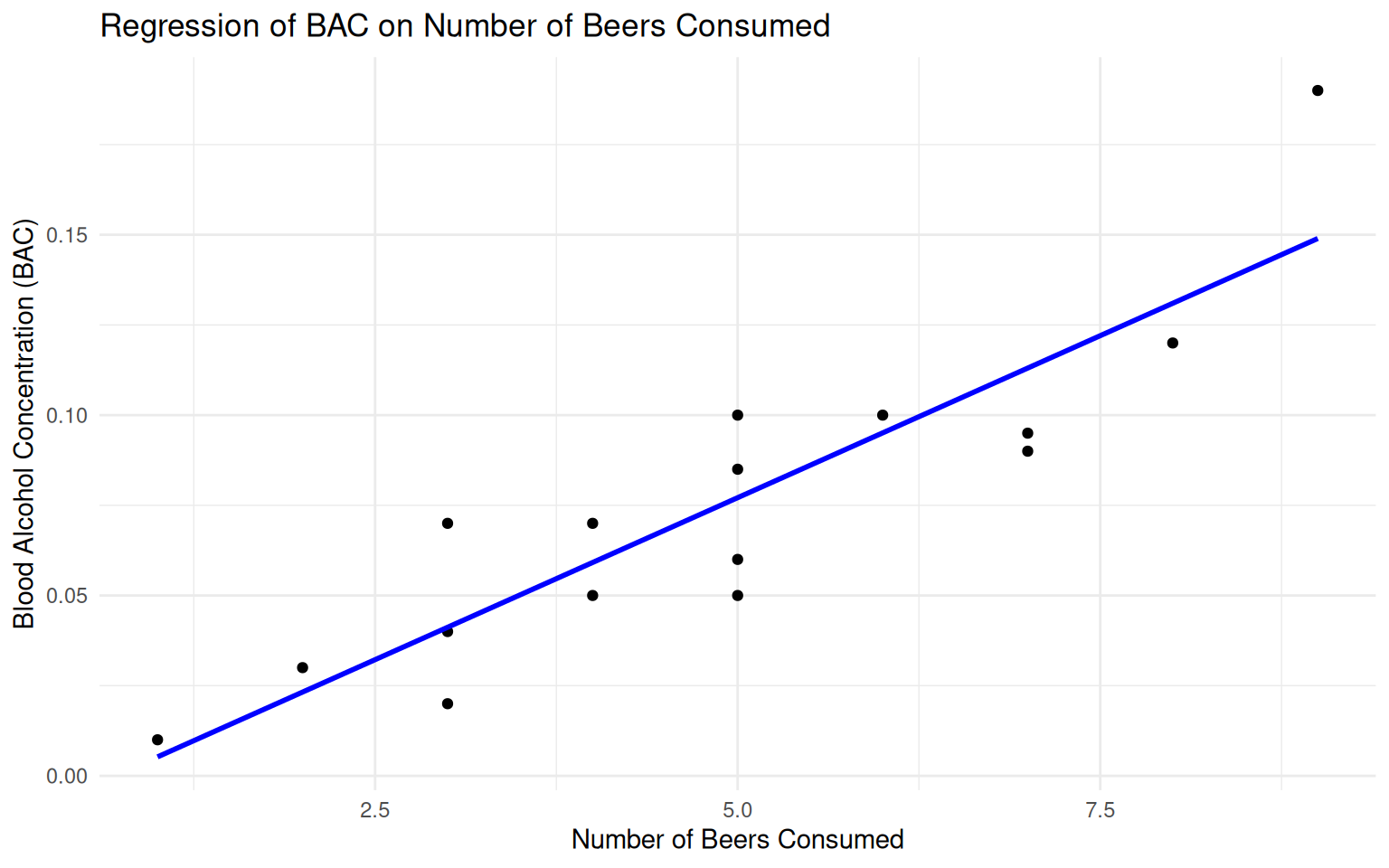
Simple Linear Regression of BAC (y) on Beers (x)

Key Question: How does beer consumption affect blood alcohol content?

\[ \begin{align*} \widehat{BAC} &=-0.0127+0.0180(\text{Beers})\\ \hat{\sigma} &= 0.02044 \end{align*} \]

Real-World Insight: Each additional beer increases BAC by about 0.018 units on average!


Call:
lm(formula = BAC ~ Beers, data = bac)

Residuals:
      Min        1Q    Median        3Q       Max 
-0.027118 -0.017350  0.001773  0.008623  0.041027 

Coefficients:
             Estimate Std. Error t value Pr(>|t|)    
(Intercept) -0.012701   0.012638  -1.005    0.332    
Beers        0.017964   0.002402   7.480 2.97e-06 ***
---
Signif. codes:  0 '***' 0.001 '**' 0.01 '*' 0.05 '.' 0.1 ' ' 1

Residual standard error: 0.02044 on 14 degrees of freedom
Multiple R-squared:  0.7998,    Adjusted R-squared:  0.7855 
F-statistic: 55.94 on 1 and 14 DF,  p-value: 2.969e-06

Confidence Interval

Key Question: How precise are our slope and intercept estimates?

\[ C\% \text{ confidence interval for } \beta_i \text{ is } \hat{\beta}_i \pm t^* \operatorname{SE}(\hat{\beta}_i) \]

Get CIs for slope/intercept with confint command or compute using qt(.975, df= ) to get t* for 95% CI

Real-World Insight: This tells us the range of plausible values for the true effect of beers on BAC!

                  2.5 %     97.5 %
(Intercept) -0.03980535 0.01440414
Beers        0.01281262 0.02311490

Inference for slope (effect of Beers on BAC)

Key Question: Is the relationship between beers and BAC statistically significant?

\[ \begin{align*} \mathrm{H}_0: &\ \beta_i = 0 & \text{(no effect for predictor i)} \\ \mathrm{H}_A: &\ \beta_i \neq 0 & \text{(predictor i has an effect on y)} \end{align*} \]

Real-World Insight: This test tells us if we’re seeing a real effect or just random variation!

term	estimate	std.error	statistic	p.value
(Intercept)	-0.0127006	0.0126375	-1.004993	0.3319551
Beers	0.0179638	0.0024017	7.479592	0.0000030

Multiple Regression Framework

Key Question: How do we extend simple regression to handle multiple predictors?

Multiple Regression Model: \[ Y = \beta_0 + \beta_1 X_1 + \beta_2 X_2 + \cdots + \beta_p X_p + \varepsilon \]
Interpretation: Each coefficient \(\beta_i\) represents the change in \(Y\) for a one-unit change in \(X_i\), holding all other predictors constant
Assumptions: Same as simple regression but extended to multiple dimensions

Real-World Insight: Multiple regression lets us control for confounding variables and understand complex relationships!

Multiple Regression Decision Framework

%%{init: {"theme": "base", "themeVariables": {"fontSize": "16px", "fontFamily": "Arial", "lineColor": "#333"}}}%%

flowchart TD
    %% --- Styling Definitions ---
    classDef start fill:#FFFACD,stroke:#FF8C00,stroke-width:3px,color:#000
    classDef decision fill:#E6F3FF,stroke:#1E88E5,stroke-width:3px,color:#000
    classDef action fill:#E8F5E9,stroke:#43A047,stroke-width:3px,color:#000
    classDef endStyle fill:#FFEBEE,stroke:#E53935,stroke-width:3px,color:#000

    %% --- Diamond Pattern Layout ---
    A["Research Question"]:::start
    
    B["Identify Predictors<br/>Select X₁, X₂, ..., Xₖ"]:::action
    
    C["Fit Multiple Regression<br/>Y = β₀ + β₁X₁ + β₂X₂ + ...+ βₖXₖ + ε<br/>where ε ~ N(0, σ²)"]:::action
    
    D["Check Assumptions"]:::decision
    
    E["t-Test Coefficients<br/>t = β̂ⱼ/SE(β̂ⱼ)<br/>H₀: βⱼ = 0"]:::action
    
    F["F-Test Overall Model<br/>F = (SSR/k)/(SSE/(n-k-1))<br/>R² = SSR/SST"]:::action
    
    G["Interpret Results<br/>95% CI: β̂ⱼ ± t*·SE(β̂ⱼ)"]:::action

    %% --- Diamond Pattern Connections ---
    A --> B
    
    B --> C
    
    C --> D
    
    D --> E
    D --> F
    
    E --> G
    F --> G

    %% --- Visual Polish ---
    linkStyle default stroke:#333,stroke-width:3px;
    linkStyle 3 stroke:#333,stroke-width:3px;
    linkStyle 4 stroke:#333,stroke-width:3px;
    linkStyle 5 stroke:#333,stroke-width:3px;
    linkStyle 6 stroke:#333,stroke-width:3px;

Scatterplot Matrix for BAC Example

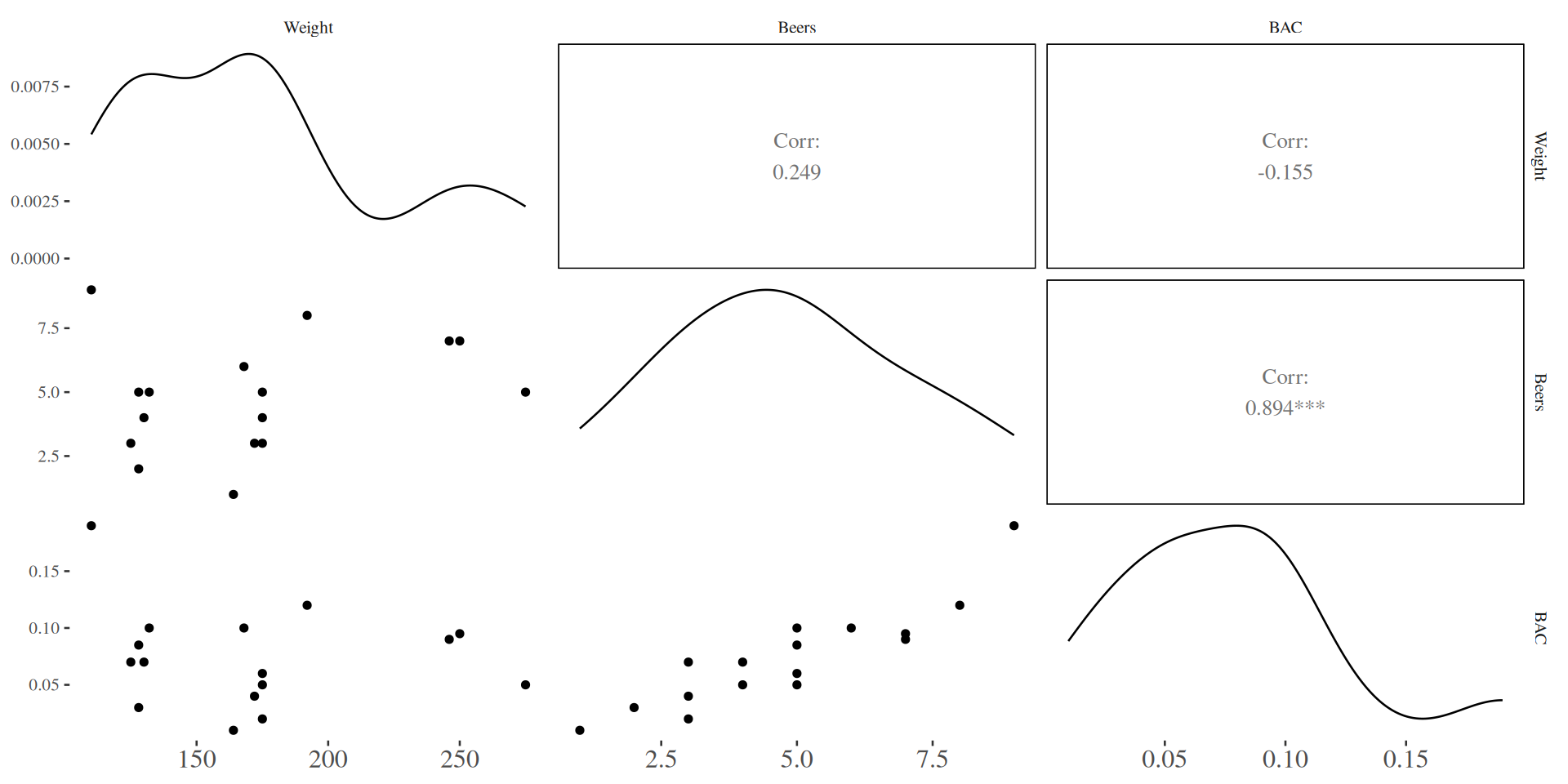
Regression of BAC on Beers and Weight

The fitted model for BAC is:


Call:
lm(formula = BAC ~ Beers + Weight, data = bac)

Residuals:
       Min         1Q     Median         3Q        Max 
-0.0162968 -0.0067796  0.0003985  0.0085287  0.0155621 

Coefficients:
              Estimate Std. Error t value Pr(>|t|)    
(Intercept)  3.986e-02  1.043e-02   3.821  0.00212 ** 
Beers        1.998e-02  1.263e-03  15.817 7.16e-10 ***
Weight      -3.628e-04  5.668e-05  -6.401 2.34e-05 ***
---
Signif. codes:  0 '***' 0.001 '**' 0.01 '*' 0.05 '.' 0.1 ' ' 1

Residual standard error: 0.01041 on 13 degrees of freedom
Multiple R-squared:  0.9518,    Adjusted R-squared:  0.9444 
F-statistic: 128.3 on 2 and 13 DF,  p-value: 2.756e-09

\[ \widehat{BAC} = 0.0399 + 0.0200 (\text{Beers}) - 0.00036 (\text{Weight}). \]

Regression of BAC on Beers and Weight

term	estimate	std.error	statistic	p.value
(Intercept)	0.0398634	0.0104333	3.820787	0.0021219
Beers	0.0199757	0.0012629	15.817343	0.0000000
Weight	-0.0003628	0.0000567	-6.401230	0.0000234

	2.5 %	97.5 %
(Intercept)	0.0173236	0.0624031
Beers	0.0172474	0.0227040
Weight	-0.0004853	-0.0002404

Regression of BAC on Beers, Weight, and Gender

Key Question: How do all three factors together predict BAC?

\[ \widehat{BAC} = 0.039 + 0.020 (\text{Beers}) - 0.00034 (\text{Weight}) - 0.0032 \text{ (Male)} \]

Real-World Insight: This model shows that gender matters too - males have slightly lower BAC than females with the same beer consumption and weight!

Both number of beers and weight are statistically significant predictors of BAC (p-value < 0.0001). Holding weight constant, we are 95% confident that the true effect of drinking one more beer is a 0.017 to 0.023 unit increase in mean BAC.

Scatterplot Matrix for BAC Example

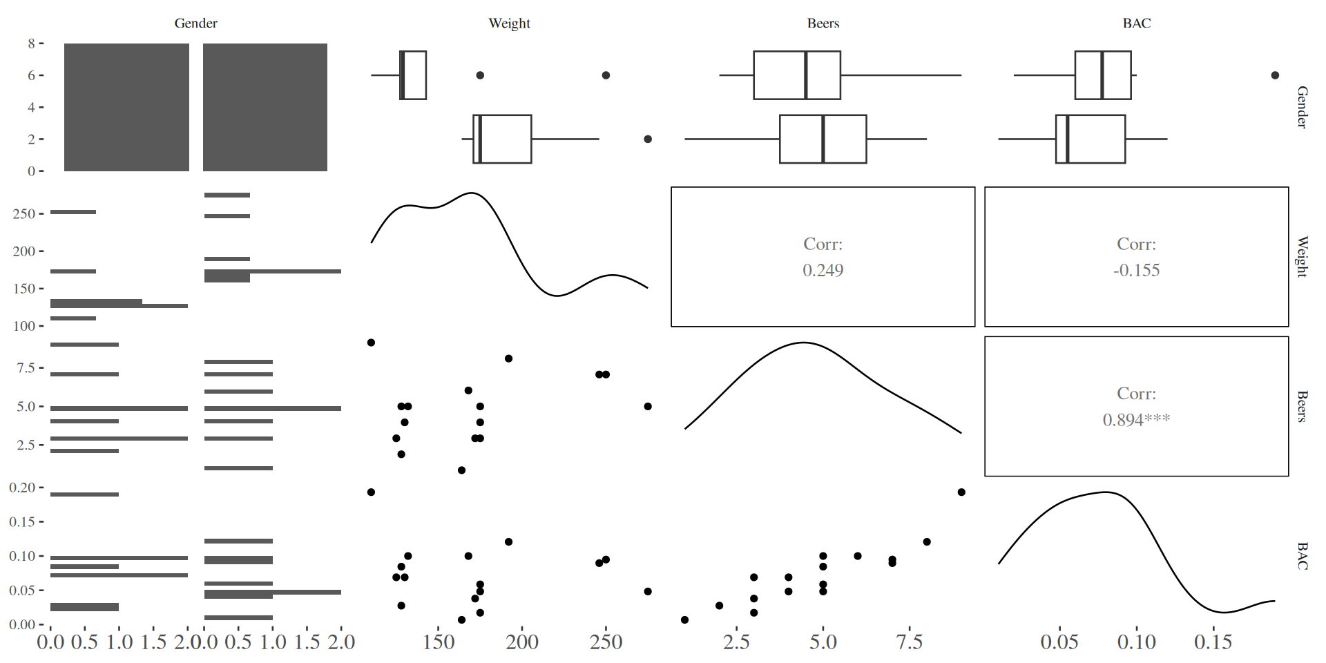
Regression for BAC on Beers, Weight, and Gender

lm2.bac <- lm(BAC ~ Beers + Weight + Gender, data = bac) # fit the model
summary(lm2.bac)


Call:
lm(formula = BAC ~ Beers + Weight + Gender, data = bac)

Residuals:
      Min        1Q    Median        3Q       Max 
-0.018125 -0.005713  0.001501  0.007896  0.014655 

Coefficients:
              Estimate Std. Error t value Pr(>|t|)    
(Intercept)  3.871e-02  1.097e-02   3.528 0.004164 ** 
Beers        1.990e-02  1.309e-03  15.196 3.35e-09 ***
Weight      -3.444e-04  6.842e-05  -5.034 0.000292 ***
Gendermale  -3.240e-03  6.286e-03  -0.515 0.615584    
---
Signif. codes:  0 '***' 0.001 '**' 0.01 '*' 0.05 '.' 0.1 ' ' 1

Residual standard error: 0.01072 on 12 degrees of freedom
Multiple R-squared:  0.9528,    Adjusted R-squared:  0.941 
F-statistic: 80.81 on 3 and 12 DF,  p-value: 3.162e-08

Regression Details for BAC on Beers, Weight, and Gender

“Male” is an indicator variable that equals 1 when predicting male Blood Alcohol Content (BAC) and 0 for female.

Barb’s Prediction
- Context: Barb drank 4 beers, weighs 160 lbs, and is female.
- Equation: \(\widehat{BAC} = 0.039 + 0.020(4) - 0.00034(160) - 0.0032(0) = 0.0646\)
John’s Prediction
- Context: John drank 4 beers, weighs 160 lbs, and is male.
- Equation: \(\widehat{BAC} = 0.039 + 0.020(4) - 0.00034(160) - 0.0032(1) = 0.0614\)

Real-World Insight: These examples show how the model accounts for individual differences - same beer consumption but different BAC predictions!

Calculation Verification

Key Question: How do we verify our multiple regression calculations in R?

Manual Prediction:

# Manual calculation verification
barb_pred_manual <- 0.039 + 0.020*4 - 0.00034*160 - 0.0032*0
john_pred_manual <- 0.039 + 0.020*4 - 0.00034*160 - 0.0032*1

# R prediction - ensure factor levels match
barb_data <- data.frame(Beers = 4, Weight = 160, Gender = factor("F", levels = levels(bac$Gender)))
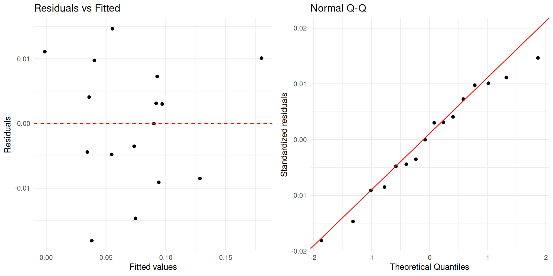
john_data <- data.frame(Beers = 4, Weight = 160, Gender = factor("M", levels = levels(bac$Gender)))

Barb's BAC:

  Manual: 0.0646

John's BAC:

  Manual: 0.0614

Day 40

Blood Alcohol Content (BAC)

Scatter Plot of BAC vs Beers

Simple Linear Regression of BAC (y) on Beers (x)

Confidence Interval

Inference for slope (effect of Beers on BAC)

Multiple Regression Framework

Multiple Regression Decision Framework

Scatterplot Matrix for BAC Example

Regression of BAC on Beers and Weight

Regression of BAC on Beers and Weight

Regression of BAC on Beers, Weight, and Gender

Scatterplot Matrix for BAC Example

Regression for BAC on Beers, Weight, and Gender

Regression Details for BAC on Beers, Weight, and Gender

Calculation Verification

Model Disgnostics