Distribution Analysis & Z-Scores
Time Allocation: 15 minutes total
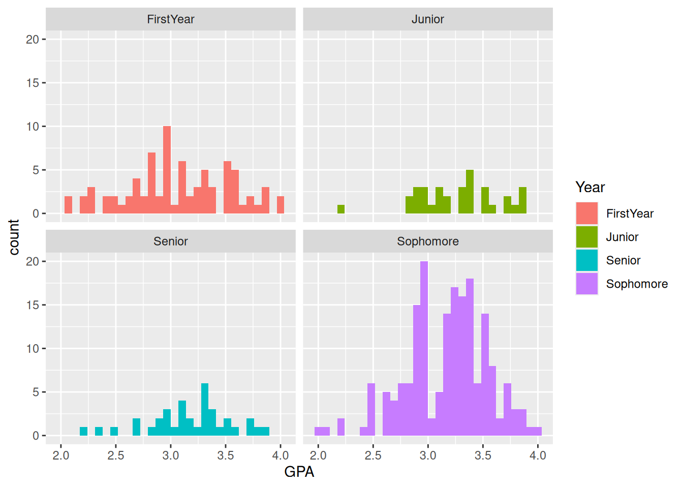
- Case Study: Use the graphical and numerical summaries of Student Survey Dataset to compare the GPA of students for different Year.
survey_data <- read.csv("https://raw.githubusercontent.com/deepbas/datasets/main/StudentSurvey.csv") |>
   tidyr::drop_na()

ggplot(survey_data, aes(x=GPA, fill=Year)) +
  geom_histogram() +
  facet_wrap(~Year)
survey_data |>
  group_by(Year) |>
  summarize(mean = mean(GPA),
            sd = sd(GPA),
            n = n()) |>
  knitr::kable(caption = "Summary Statistics of GPA for all Years")
Summary Statistics of GPA for all Years
| FirstYear |
3.070759 |
0.4702584 |
79 |
| Junior |
3.273636 |
0.3688057 |
33 |
| Senior |
3.171667 |
0.3754274 |
36 |
| Sophomore |
3.173224 |
0.3690737 |
183 |
Part 1: Distribution Concepts (5 minutes)
Instructions: Provide examples and explanations for each concept:
Symmetric Distribution Example: _________________________
- Why it’s symmetric: ____________________________________
Real-world skewed distribution: _________________________
- Direction of skew: □ Left □ Right
- Reason for skew: ______________________________________
Normal distribution characteristic: ______________________
Part 2: Z-Score Interpretation (5 minutes)
Scenario: A student’s GPA has a z-score of 2.
What does this mean?
- □ GPA is 2 points above mean
- □ GPA is 2 standard deviations above mean
- □ GPA is 2 standard deviations below mean
- □ GPA is 2 points below mean
Explanation: __________________________________________
If mean GPA = 3.0 and SD = 0.5, calculate actual GPA:
- Formula: _________________________
- Calculation: ______________________
- Actual GPA: ______________________
Part 3: Data Analysis (5 minutes)
Analysis Questions:
Which year has the highest average GPA? __________________
Potential explanation for this pattern:
Two potential biases in this dataset: